A free update to Stata 13 is available

Oct/Nov/Dec

Vol 28 No 4

The Stata News

Executive Editor ............Karen Strope

Production Supervisor ... Annette Fett

Censored outcomes

If you analyze data with Gaussian

dependent variables that are censored,

you will want to update to Stata 13.1.

You can now do just about anything you

want with such outcomes. Extensions

of tobit and censored regression models

include the following:

• Selection models

• Random effects and coefﬁcients

• Endogenous covariates

• Treatment effects (ATEs)

• Multivariate models

• Unobserved components

• Endogenous switching models

All of these models may be combined

with each other. For example, you

can specify a tobit model with random

effects, random coefﬁcients, sample

selection, and endogenous covariates.

Moreover, the random coefﬁcients

can occur in both the outcome and

selection models.

All of these features are implemented

through extensions to Stata’s gsem

(generalized SEM) command and

graphical SEM Builder.

See page 3 for a discussion.

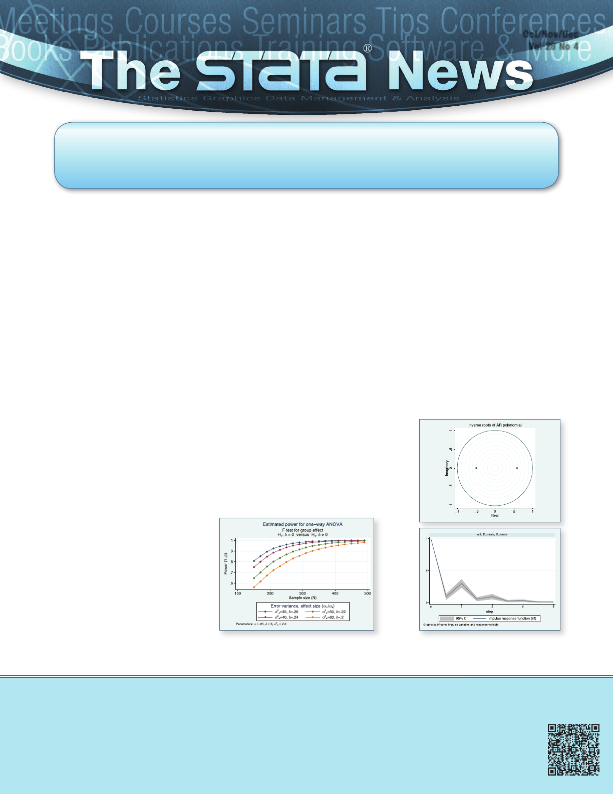
Power and sample size

The power command that was

introduced in Stata 13 has new methods

for analysis of ANOVA models:

• One-way models

• Two-way models

• Repeated-measures models

Like other power methods, you can

compute (1) sample size, (2) power, or

(3) effect size. Compute any of the

three given the other two.

You just tell power what you know,

and it produces tables and graphs of

what you want to know.

Stata 13.1 also introduces facilities

to easily add your own new methods

to the power command and

produce tables and graphs of results

automatically.

See page 2 for details.

Time series

Stata 13.1 also adds several new

features for the analysis of univariate

time series:

• IRFs (impulse–response functions)

for ARIMA and ARFIMA models

• Autocorrelation functions from

ARIMA and ARFIMA models

• Parametric spectral densities for

seasonal ARIMA models

• Stability checks for ARIMA models

All of your favorite multivariate tools

can now be applied to univariate models.

See page 4 to see these features.

Haven’t upgraded to Stata 13 yet?

You’re missing one of the most exciting releases of Stata ever. Learn more on page 8.

A free update to Stata 13 is available—Stata 13.1

For those who have Stata 13, just type update query in Stata, and follow the instructions, or

select “Check for updates” from the Help menu. Stata 13.1 introduces several new features.

New power and sample size for ANOVA .... 2

New features for censored outcomes and

tobit models ................................................. 3

In the spotlight: New univariate time-series

features added in 13.1 ................................. 4

New distribution functions .......................... 5

In the spotlight: Adding your own methods

to analyze power and sample size ............. 6

Stata Conference Boston 2014 ................... 9

Visit us at ASSA 2014 .................................. 9

Econometrics Winter School using Stata ... 9

Public training courses ............................. 10

NetCourses™ ............................................ 10

New from Stata Press ............................... 11

New from the Stata Bookstore ................. 11

Stata 13.1, a free update to Stata 13, adds three new

methods for power and sample-size analysis of ANOVA

models—oneway, twoway, and repeated:

• power oneway

performs analyses for one-way ANOVA

• power twoway

performs analyses for two-way ANOVA

• power repeated

performs analyses for repeated-measures ANOVA

These new facilities work just like the existing facilities

for comparisons of means, proportions, correlations, and

variances. You can specify single values or ranges of values

for power and effect size to compute required sample size.

You can specify sample size and effect size to compute

power. Or you can specify power and sample size to

compute effect size.

Your results can be displayed either in tabular form or as a graph.

Multiple scenarios can be compared on a table or a graph.

For one-way ANOVA, you can perform analyses either on

comparisons of means or on arbitrary contrasts of means.

All methods work with unbalanced models.

You can specify your problem in the way you ﬁnd most

convenient. For example, to compute the required sample

size for a one-way analysis, you can specify the projected

group means directly, or you can specify between-group

variability. power oneway will accommodate either of

these speciﬁcations.

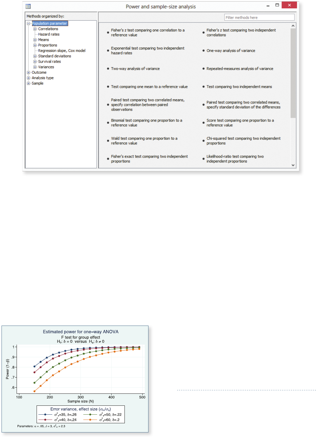
You can perform your analysis using

either natural command syntax (see

stata.com/stata13/power-and-sample-size) or

the integrated power and sample-size control panel—a

graphical interface to guide you through your analysis.

Read about all the new features provided for power

and sample-size analysis in Stata 13 and 13.1 at

stata.com/stata13/power-and-sample-size. There

you will ﬁnd highlights and a quick overview of the new

features, links to videos, links to worked examples, and

even a PDF of the new Power and Sample-Size Reference

Manual.

New power and sample size for ANOVA

We can even add a random coefﬁcient on age by interacting a random latent variable (RC[id]) with age:

. gsem (income <- education age c.age#RC[id] weeks UC RE[id], family(gaussian, rcensored(150000)))

(weeks <- education age z1 z2 UC@1 , var(UC@1))

New features for censored outcomes and tobit models

We often cannot observe or measure an outcome over its full range. Tests for detecting a toxin often require the toxin to

exceed a threshold before it can be detected—left-censoring. Patients’ weights will be censored at the upper limit of the

scale used to weigh them—right-censoring.

Related to left- and right-censoring are interval measurements, or interval censoring. Income can be surveyed in ranges ($0

to $10,000, $10,001 to $30,000, $30,001 to $60,000, $60,001 and up), or patient weight can be recorded in ranges (0–80

pounds, 81–120 pounds, 121–150 pounds, 151–180 pounds, 181–220 pounds, 221–250 pounds, over 250 pounds).

Stata has long been able to estimate regression models with censored outcomes. tobit can estimate models with left- or

right-censoring at ﬁxed values. intreg can estimate models with interval measurements or censoring that varies across

observations.

New with the Stata 13.1 update, you can now estimate models with censored or interval-measured Gaussian outcomes

that also include Heckman-style selection, endogenous treatments to obtain average treatment effects (ATEs), covariate

measurement error, and unobserved components. You can include endogenous regressors in any part of the models. You

can also estimate these models in a panel-data or multilevel-data context with random effects (intercepts) and random

coefﬁcients in any part or all parts of the model. All of these models can be estimated as parts of larger multivariate

systems. Censored or interval-measured outcomes can even participate in endogenous switching models.

Imagine we have data on incomes. These data are often top coded, or censored at an upper limit, to increase reporting

rates. If that limit were $150,000, we could estimate a regression model of income on education and age by typing

. tobit income education age, ul(150000)

(We might prefer log income, but for simplicity, we will use income here.)

All the new features are obtained using Stata 13’s generalized structural equation modeling command—gsem. The

equivalent gsem command is

. gsem income <- education age, family(gaussian, rcensored(150000))

We can introduce an endogenous covariate, say, weeks worked, by adding an equation for weeks with instruments

(z1 and z2) and a common unobserved component (UC) with identifying constraints speciﬁed using @:

. gsem (income <- education age weeks UC, family(gaussian, rcensored(150000)))

(weeks <- education age z1 z2 UC@1 , var(UC@1))

If we have panel data with repeated measurements on individuals (id), we can introduce a random effect (intercept) into

the income model by adding RE[id]:

. gsem (income <- education age weeks UC RE[id], family(gaussian, rcensored(150000)))

(weeks <- education age z1 z2 UC@1)

Continued on next page.

In the spotlight: New univariate time-series features added in 13.1

Stata 13.1 introduces four new features for univariate

time series:

1. IRFs (impulse–response functions) for ARIMA and

ARFIMA models

2. Parametric autocorrelation estimates from ARIMA

and ARFIMA models

3. A check of stability conditions for ARIMA models

4. Spectral density estimation from seasonal ARIMA

models

Individually, none of these features are earth shattering.

However, the ﬁrst three are some of my go-to concepts

when teaching time-series analysis. Let’s use an example

to see why.

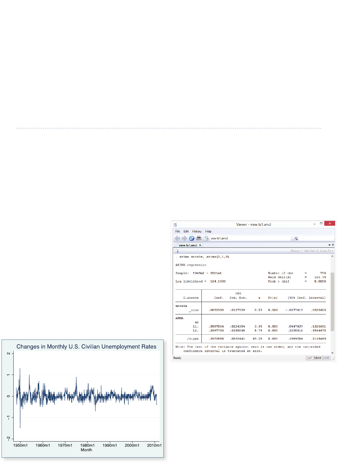
Here is a graph of changes in monthly U.S. civilian

unemployment rates for the period 1948–2011.

The AR parameters are statistically signiﬁcant, and they

indicate a moderate degree of temporal dependence.

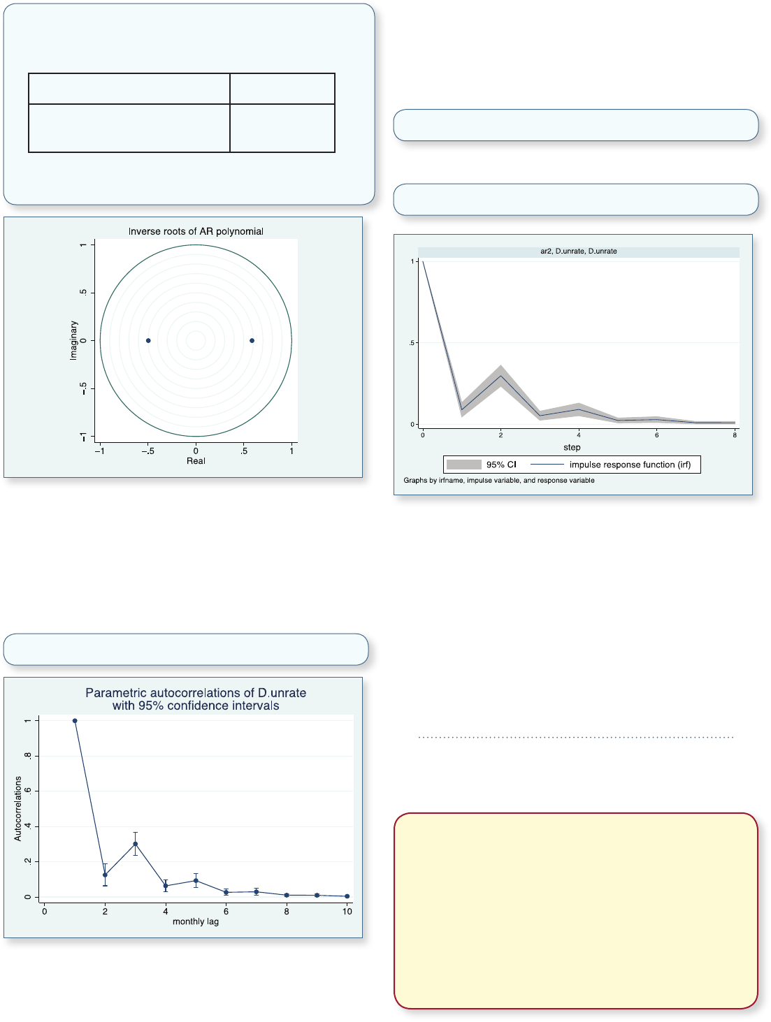
Inference after ARIMA requires that the ARMA

(autoregressive moving-average) process be covariance

stationary. The stationarity of an ARMA process depends

on the AR parameters. The inverse roots of the AR

polynomial must all lie inside the unit circle for the

process to be stationary. We use the new estat aroots

command to examine this requirement:

Handling Heckman-style selection in the gsem framework requires a bit of setup. See

stata.com/manuals13/semexample45g.pdf for an example using an uncensored outcome variable. For censored

outcomes, you merely need to add the suboption lcensored() or rcensored() to the family() option.

An endogenous treatment-effects example without censoring can be found at

stata.com/manuals13/semexample46g.pdf. Again just add lcensored() or rcensored() to family() if the outcome

is censored.

You can use either the commands shown above or Stata’s SEM Builder to create and estimate these models.

Stata 13.1 provides everything you could want with censored outcomes.

Read about the other new features provided by generalized SEM at stata.com/stata13/generalized-sem. There you

will ﬁnd an overview of SEM and generalized SEM, links to videos, links to worked examples, and even the full PDF of

Stata 13’s Structural Equation Modeling Reference Manual.

We ﬁt an ARIMA model with two autoregressive (AR)

terms, ﬁrst-differencing, and no moving-average terms.

. estat aroots

Eigenvalue stability condition

+----------------------------------------+

| Eigenvalue | Modulus |

|--------------------------+-------------|

| .5844888 | .584489 |

| -.4957824 | .495782 |

+----------------------------------------+

All the eigenvalues lie inside the unit circle.

AR parameters satisfy stability condition.

The ARMA process appears to be stationary because both

inverse AR roots lie well inside the unit circle.

A crucial aspect of time-series processes are their

autocorrelations. The autocorrelations provide a scale-free

measure of the dependence structure of the process. We

can obtain a graph of this structure using the new estat

acplot command after estimating our ARIMA model:

. estat acplot, lags(10)

The graph shows that the autocorrelations decay

exponentially toward 0, which is typical of a stationary

AR process with positive coefﬁcients.

We often want to know how an exogenous shock feeds

through our model and affects the series. This response,

measured over time, is called the impulse–response

function (IRF).

We create an IRF for our ARIMA model by typing

. irf create ar2, set(myirf)

and then graph that IRF by typing

. irf graph irf

The trajectory of the IRF shows that a positive shock

initially causes an increase in unemployment but that the

increase nears 0 by 5 months and completely dies out after

7 or 8 months.

You can see more examples of these new facilities

in the manuals. See arima postestimation

(stata.com/manuals13/tsarimapostestimation.pdf)

and arﬁma postestimation

(stata.com/manuals13/tsarﬁmapostestimation.pdf).

- Rafal Raciborski

Senior Statistical Developer

New distribution functions

Stata 13.1 adds three new functions that compute

aspects of the noncentral chi-squared distribution:

nchi2den() density

nchi2tail() reverse cumulative

invnchi2tail() inverse of reverse cumulative

In the spotlight: Adding your own methods to analyze power and

sample size

Stata 13 added a suite of power commands to analyze power

and sample size. Stata 13.1 extends that suite to ANOVA.

In some cases, you may want to compute sample size or power

yourself. For example, you may need to do this by simulation,

or you may want to use a method that is not available in any

software package. power makes it easy for you to add your

own method. All you need to do is to write a program that

computes sample size, power, or effect size, and the power

command will do the rest for you. It will deal with the support

of multiple values in options and with automatic generation of

graphs and tables of results.

Suppose you want to add the method called mymethod to the

power command. Just follow these three steps:

1. Create a program that computes sample size, power, or

effect size and follows power’s naming convention—

power_cmd_mymethod.ado.

2. Store results following power’s simple naming

conventions for results. For example, store the value of

power in r(power), the value of sample size in r(N), and

so on.

3. Place your program power_cmd_mymethod.ado where

Stata can ﬁnd it.

To show how easy this all is, we’ll write an ado program to

compute power for a one-sample z test given sample size,

standardized difference, and signiﬁcance level. For simplicity, we

assume a two-sided test.

We will call our new method myztest.

program power_cmd_myztest, rclass

version 13.1

// parse options

syntax , n(integer) /// sample size

STDDi(real) /// standardized di.

Alpha(string) /// signicance level

// compute power

tempname power

scalar `power’ = normal(`stddi’*sqrt(`n’) - ///

invnormal(1-`alpha’/2))

// return results

return scalar power = `power’

return scalar N = `n’

return scalar alpha = `alpha’

return scalar stddi = `stddi’

end

The computation in this program takes only one line,

but it could be as complicated as we like. It could

even involve simulation to compute the power.

With our program in hand, we can type

. power myztest, n(20) stddi(1) alpha(.05)

power will ﬁnd our ado program, supply it with the

options n(20), stddiff(1), and alpha(.05), and use its

returned results to produce

. power myztest, n(20) stddi(1) alpha(.05)

Estimated power

Two-sided test

+-------------------------+

| alpha power N |

|-------------------------|

| .05 .994 20 |

+-------------------------+

That wasn’t too impressive. Our program did all the work.

But what if we supplied power with a list of sample

sizes?

. power myztest, n(10 15 20 25) stddi(1)

Estimated power

Two-sided test

+-------------------------+

| alpha power N |

|-------------------------|

| .05 .8854 10 |

| .05 .9721 15 |

| .05 .994 20 |

| .05 .9988 25 |

+-------------------------+

power has taken our list of sample sizes and computed

powers for all of them—even though our program

could only compute a single power!

Moreover, we can use power’s standard table() option

to control exactly how that table looks. power also

has hooks that let our program determine how the

columns are labeled and how the table appears.

We can supply both sample sizes and signiﬁcance

levels and request a graph instead of a table:

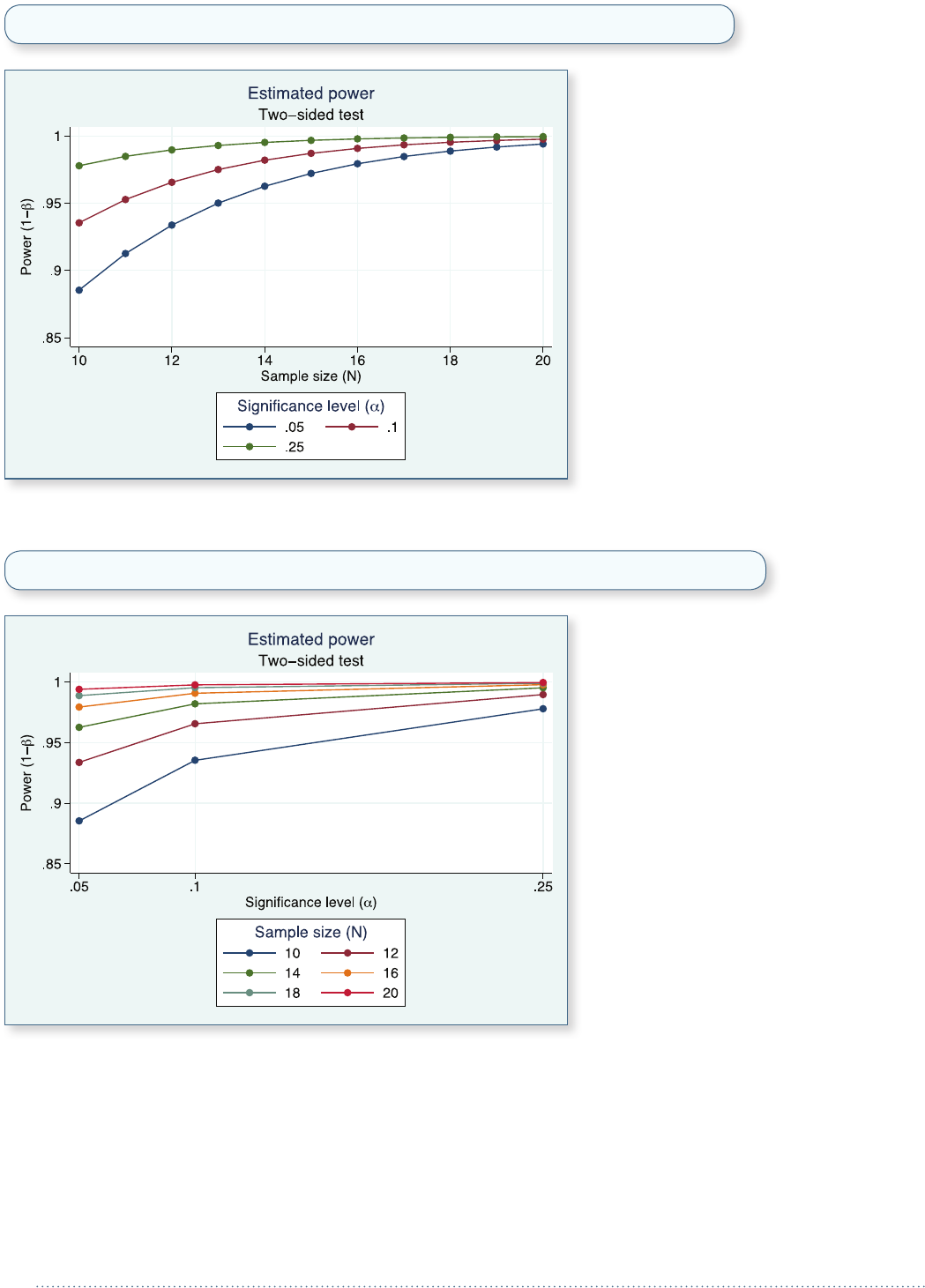
. power myztest, n(10(1)20) alpha(.05 .10 .25) stddi(1) graph

We can even request that the graph show α on the x axis with separate plots for each sample size.

. power myztest, n(10(2)20) alpha(.05 .10 .25) stddi(1) graph(xdim(alpha))

Now all this may just make it worth writing more complicated programs to compute power for more complicated tests

and comparisons.

We had room here to do just a simple example. More details and extensions of this example are covered in my

presentation at the 2013 UK Stata Users Group meeting —

stata.com/meeting/uk13/abstracts/materials/uk13_marchenko.pdf. Complete documentation for user-

programmed power and sample size can be found in Stata 13.1 by typing help power userwritten.

- Yulia Marchenko

Director of Biostatistics

Stata 13 adds features and statistics for virtually every user in every ﬁeld. Here are the highlights.

Treatment effects

You can now estimate the effect of treatments such as a new drug regimen, a surgical procedure, or a

training program using inverse-probability weights (IPW), propensity-score matching, doubly robust

methods, and other techniques. Your treatment can be binary, multilevel (for example, four dosages of the

same drug), or multivalued (for example, four different drugs).

Multilevel models and panel data

Need to handle binary, ordered, count, and categorical outcomes in panel or repeated-measures data? Stata’s extensive

multilevel and panel-data modeling facilities have been extended to include probit, negative binomial, ordered logistic,

ordered probit, and multinomial logistic—all with cluster–robust SEs.

Generalized SEM

Tired of just linear SEMs? Stata 13 adds multilevel nested and crossed models. We also add support

for binary, count, categorical, and ordered outcomes. With these new features, you can estimate a

dizzying array of models—multilevel CFA with ordinal measurements, multilevel mediation, item-

response theory (IRT) ... any multilevel SEM with generalized linear outcomes.

Power and sample size

Perform power and sample-size analyses from an integrated Control Panel. Get tables, graphs, or

both at the click of a button. Enter lists of known or possible values, and solve for power, sample

size, minimum detectable effect, or effect size.

Forecasting

Estimate any number of models—regressions, simultaneous systems, VARs, etc.—and produce time-series forecasts from

all the estimates. Create dynamic or static (one-step ahead) forecasts. Apply add factors and other adjustments, specify

identities, and compare alternative scenarios—even produce conﬁdence intervals via stochastic simulation.

Long strings

Maximum string length increases from 244 characters to 2 billion! Stata also now handles binary large objects (BLOBs)

such as Word documents and JPEG images. These long strings work just as strings have always worked in Stata—all

functions and commands work with them.

Project Manager

Keep all of your ﬁles associated with a Stata project in one place. Filter on ﬁlename, and click

to open or run do-ﬁles, ado-ﬁles, datasets, raw ﬁles, graphs, etc. Create groups to categorize

ﬁles. Create any number of projects that pass seamlessly across all of your computers, even

across different operating systems.

And there are many more substantial additions, such as effect size, Poisson regression with endogenous regressors, probit

with sample selection, and import delimited with preview.

Upgrade now at stata.com/stata13.

Econometrics Winter School

using Stata

Philadelphia, Pennsylvania

January 3–5, 2014

The Allied Social Science Association (ASSA) will

have its annual meeting in Philadelphia, Pennsylvania,

from January 3–5. For more information, visit

aeaweb.org/Annual_Meeting.

Stata representatives, including David M. Drukker,

Director of Econometrics, will be on hand to answer

your questions on all things Stata. Stop by booth #405

to visit with the people who develop and support the

software.

We’re interviewing at ASSA! Go to

stata.com/careers/assa14. Submit your completed

application before December 16, 2013, and let us know

that you would like to be considered for an interview at

the meetings.

Visit us at ASSA 2014

Timberlake (Portugal) and the Faculty of Economics at

the University of Porto are jointly organizing a set of

applied econometrics courses using Stata. The aim of these

courses is to familiarize the participants with the basic

econometric tools commonly used in applied research.

The courses include a quick discussion of the relevant

econometric theory as well as an in-depth discussion of

empirical applications using real data. The courses, taught

in English, will take place at FEP, University of Porto, on

January 21–24, 2014.

Available courses

Day 1: Data management and regression analysis (OLS, GLS)

Day 2: IV and panel-data models

Day 3: Discrete choice models

Day 4: Duration models

For more information or to register, visit Timberlake’s

website at www.timberlake.pt/landings/v9.

When July 31–August 1, 2014

Where Omni Parker House

60 School Street

Boston, Massachusetts

Details

stata.com/boston14

Conference Boston 2014

Come join us in historic Boston, home to Fenway Park

and the Harvard Museum of Natural History, for two

days of networking and Stata exploration. Don’t miss

this opportunity to connect with colleagues and fellow

researchers, as well as Stata developers.

Call for presentations

All users are encouraged to submit abstracts for possible

presentations, which can address any Stata-related topic,

including the following:

• New user-written commands, including commands

for modeling and estimation, graphical analysis, data

management, or reporting

• Use or evaluation of existing Stata commands

• Methods for teaching statistics with Stata or teaching

the use of Stata

• Case studies of Stata use in novel areas or applications

• Surveys or critiques of Stata facilities in speciﬁc ﬁelds

• Comparisons of Stata with other software or use of

Stata together with other software

Each user presentation should be either 15 or 25 minutes

long and should be followed by 5 minutes for questions.

Longer presentations will be considered at the discretion

of the scientiﬁc committee.

For submission guidelines, visit stata.com/boston14.

Submissions are due by February 21, 2014.

Scientiﬁc committee

• Stephen Soldz (Chair)

Boston Graduate School of Psychoanalysis

• Kit Baum

Boston College

• Marcello Pagano

Harvard University

Whether you stay for the JSM or just to relax, be sure to

enjoy what Boston has to offer. Take a cruise in Boston

Harbor, walk the Freedom Trail, visit Fenway Park, and

have a bowl of “chowdah”. Boston is a great city with

plenty to do and see.

NetCourses™

NetCourses are convenient web-based courses that teach

you how to exploit the full power of Stata.

Introduction to Survival Analysis

Using Stata

Intended for everyone who uses Stata to perform survival

analysis, whether health researchers or social scientists,

the course includes an introduction to concepts such

as censoring, truncation, hazard rates, and survival

functions. The remainder of the course focuses on the

analysis of survival data. Topics include data preparation,

descriptive statistics, life tables, Kaplan–Meier curves,

and semiparametric (Cox) regression and parametric

regression. Exercises are included to reinforce the course

material. Some familiarity with Stata is important, but no

prior knowledge of survival analysis is necessary.

Dates: January 17–March 7, 2014

Cost: $295

Public training courses

Public training courses are intensive, in-depth courses taught by StataCorp at a third-party site.

Using Stata Effectively: Data Management, Analysis, and Graphics Fundamentals

January 7–8, 2014, Washington, DC

Aimed at both new Stata users and those who wish to learn techniques for efﬁcient day-to-day use of Stata, this course

enables you to use Stata in a reproducible manner, making collaborative changes and follow-up analyses much simpler.

Exercises will supplement the lectures and Stata examples.

Estimating Average Treatment Effects Using Stata

March 6–7, 2014, Washington, DC

This course discusses methods in Stata that use observational data to estimate average treatment effects and average

treatment effects on the treated. We will cover the conceptual and theoretical underpinnings of treatment effects as well

as many examples using Stata.

Structural Equation Modeling Using Stata

March 24–25, 2014, Washington, DC

Learn how to illustrate, specify, and estimate structural equation models in Stata using both Stata’s SEM Builder and the

sem command. The course introduces several types of models, including path analysis, conﬁrmatory factor analysis, full

structural equation models, and latent growth curves. Exercises supplement the lessons and Stata examples.

Multilevel/Mixed Models Using Stata

April 23–24, 2014, Washington, DC

Measure and account for clustering and grouping at multiple levels. Whether linear or nonlinear, multilevel modeling

allows for random intercepts and slopes at multiple levels, reducing the problems of too-much or too-little data

aggregation. The course is interactive, uses real data, offers ample opportunity for speciﬁc research questions, and provides

exercises to reinforce what you learn.

Find out more at stata.com/public-training.

NEWNEW

Don’t forget our other courses!

Introduction to Stata

Dates: January 17–February 28, 2014

Cost: $95

Introduction to Stata Programming

Dates: January 17–February 28, 2014

Cost: $125

Advanced Stata Programming

Dates: January 17–March 7, 2014

Cost: $150

Introduction to Univariate Time Series Using Stata

Dates: January 17–March 7, 2014

Cost: $295

stata.com/netcourse

The dates above don’t work for you? No problem!

NetCourseNow allows you to set the schedule. Visit

stata.com/netcourse/ncnow.

More titles online!

The Stata Bookstore contains nearly 200 titles, all carefully

selected to meet the needs of our users. Check out the

Bookstore online at stata.com/bookstore.

New from the Stata Bookstore

Applied Logistic Regression, Third Edition

Authors: David W. Hosmer, Jr.,

Stanley Lemeshow,

and Rodney X.

Sturdivant

Publisher: Wiley

ISBN-13: 978-0-470-58247-3

Pages: 528; hardcover

Price: $94.75

The third edition of Applied Logistic Regression, by David

W. Hosmer, Jr., Stanley Lemeshow, and Rodney X.

Sturdivant, is the deﬁnitive reference on logistic regression

models.

Most of the analyses in the book were performed using

Stata and can be replicated using Stata and the data from

the text. Also noteworthy is the book’s use of multinomial

fractional polynomial models that can be ﬁt using Stata’s

mfp command.

Read more or order online at

stata.com/bookstore/applied-logistic-regression.

Applied Longitudinal Data Analysis for

Epidemiology: A Practical Guide, Second

Edition

Author: Jos W. R. Twisk

Publisher: Cambridge University

Press

ISBN-13: 978-1-107-69992-2

Pages: 321; paperback

Price: $59.50

Applied Longitudinal Data Analysis for Epidemiology: A

Practical Guide, Second Edition, by Jos W. R. Twisk, provides

a practical introduction to the estimation techniques used

by epidemiologists for longitudinal data.

Read more or order online at

stata.com/bookstore/longitudinal-data-analysis-epidemiology.

Econometric Analysis of Panel Data,

Fifth Edition

Author: Badi H. Baltagi

Publisher: Wiley

ISBN-13: 978-1-118-67232-7

Pages: 390; paperback

Price: $59.75

Econometric Analysis of Panel Data, Fifth Edition, by

Badi H. Baltagi, is a standard reference for performing

estimation and inference on panel datasets from an

econometric standpoint. This book provides a rigorous

introduction to standard panel estimators as well as concise

explanations of many newer, more advanced techniques.

Because of its wide range of topics and detailed

exposition, Econometric Analysis of Panel Data, Fifth Edition,

can serve as both a graduate-level textbook and a handy

desk reference for seasoned researchers.

Read more or order online at

stata.com/bookstore/econometric-analysis-of-panel-data.

New from Stata Press

Discovering Structural Equation Modeling

Using Stata, Revised Edition

Author: Alan C. Acock

ISBN-13: 978-1-59718-139-6

Pages: 306; paperback

Price: $48.00

Discovering Structural Equation Modeling Using Stata, Revised

Edition is an excellent resource both for those who are

new to SEM and for those who are familiar with SEM

but new to ﬁtting these models in Stata. It is useful as a

text for courses covering SEM as well as for researchers

performing SEM.

The Revised Edition includes output, syntax, and

instructions for ﬁtting models with the SEM Builder that

have been updated for Stata 13.

Read more or order online at

stata-press.com/discovering-sem.

979-696-4600 979-696-4601 (fax)

ser[email protected] stata.com

Please include your Stata serial number with all correspondence.

Find a Stata distributor near you

stata.com/worldwide

StataCorp

4905 Lakeway Drive

College Station, TX 77845-4512

USA

Return service requested.

/StataCorp /Stata

blog.stata.com

/StataCorp

/+Stata

Go green!

The Stata News is now available via email.

Be eco-friendly and go paperless.

Have the Stata News delivered straight to your inbox.

electronic format before it arrives in the mail. We will

send you an email with the News content as soon as it is

available. The electronic format of the Stata News has all

the same information as the printed version. The only

difference is the convenience.

Go to

stata.com/news-delivery

to choose your delivery method.

Select email, printed, or both.

Get your News your way.