
Longitudinal Data Analysis by Example
Fares Qeadan, Ph.D
Department of Internal Medicine
Division of Epidemiology, Bi ostatis tics, & Preventive Medicine
University of New Mexico Health Sciences Center
April 5, 2016
Fares Qeadan, Ph.D (Department of Internal Medicine Division of Epidemiology, Biostatistics, & Preventive MedicineUniversity of New Mexico Health Sciences Center)Longitudinal Data Analysis by Example April 5, 2016 1 / 31

Outline
Longitudinal Data Analysis
Definitions: Longitudinal vs. Time series
Data Structure
Properties of Longitudinal Data
Graphical visualization
Modeling strategies
Mixed Effects Modeling
Model selection
Example: Beating the Blues
Background
Research Questions
Selecting the Covariance Structure
Analysis for Research Questions
Pitfalls
Inference on Individuals
References
Citation
Fares Qeadan, Ph.D (Department of Internal Medicine Division of Epidemiology, Biostatistics, & Preventive MedicineUniversity of New Mexico Health Sciences Center)Longitudinal Data Analysis by Example April 5, 2016 2 / 31

Longitudinal Data Analysis Definitions
Longitudinal Studies:
Studies in which subjects’ outcomes and possibly treatments or exposures
are measured at multiple follow-up times and thus their statistical analysis
constitutes an analysis of intra- and inter-individual variation [1].
Results generalize across the population from which the sample of
subjects was drawn
Example: A study in which 66 patients have their Depression Scores
measured at baseline (before treatment), and weekly for the next 5 weeks.
Time Series Studies:
Studies that pertain to the sequential behavior of a single subject (or any
unitary entity) and thus their statistical analysis constitutes an analysis of
intra-individual variation [2].
Results do not generalize across some population of subjects but
instead generalize across the time domain.
Example: Studying the number of Upper Urinary Tract Stones among
adults in New Mexico ove r time.
Fares Qeadan, Ph.D (Department of Internal Medicine Division of Epidemiology, Biostatistics, & Preventive MedicineUniversity of New Mexico Health Sciences Center)Longitudinal Data Analysis by Example April 5, 2016 3 / 31
Longitudinal Data Analysis Definitions
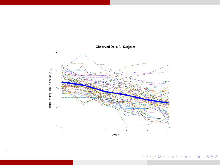
Standard plot from Longitudinal data: Spaghetti plot of individual
patient-specific longitudinal relationships between Hamilton Depression
Scores (HD) and time for each subject
1
.
1
This figure was generated from a data set taken from [3].
Fares Qeadan, Ph.D (Department of Internal Medicine Division of Epidemiology, Biostatistics, & Preventive MedicineUniversity of New Mexico Health Sciences Center)Longitudinal Data Analysis by Example April 5, 2016 4 / 31
Longitudinal Data Analysis Definitions
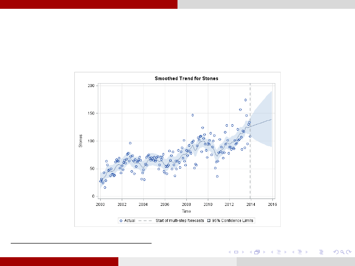
Standard plot from a Time Series data: Plot of the number of Upper
Urinary Tract Stones by time for adults in New Mexico through the UNM
network
2
.
2
This figure was generated from a data set taken from [4].
Fares Qeadan, Ph.D (Department of Internal Medicine Division of Epidemiology, Biostatistics, & Preventive MedicineUniversity of New Mexico Health Sciences Center)Longitudinal Data Analysis by Example April 5, 2016 5 / 31
Longitudinal Data Analysis Data Structure
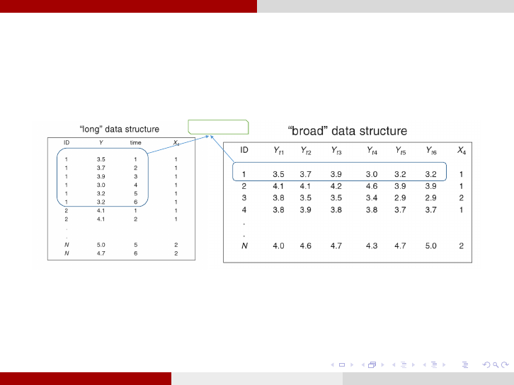
Data Structure for Longitudinal Studies: Longitudinal data files have
two types of structure (Long and Wide). However, usually wide (broad)
format (one row per subject) are converted to long format (one row for
each time point by subject combination)[5].
Data for subject 1
Remark 1.Longitudinal data, that follow one subject’s changes over the course of time
make a time series.
Remark 2.Longitudinal data generally are associated with a limited number of time
p oi nts whereas time series data can entail a large number of repetitive occasions [6].
Fares Qeadan, Ph.D (Department of Internal Medicine Division of Epidemiology, Biostatistics, & Preventive MedicineUniversity of New Mexico Health Sciences Center)Longitudinal Data Analysis by Example April 5, 2016 6 / 31

Longitudinal Data Analysis Data Structure
Data Structure for Longitudinal Studies: Longitudinal data files have
two types of structure (Long and Wide). However, usually wide (broad)
format (one row per subject) are converted to long format (one row for
each time point by subject combination)[5].
Data for subject 1
Remark 1.Longitudinal data, that follow one subject’s changes over the course of time
make a time series.
Remark 2.Longitudinal data generally are associated with a limited number of time
p oi nts whereas time series data can entail a large number of repetitive occasions [6].
Fares Qeadan, Ph.D (Department of Internal Medicine Division of Epidemiology, Biostatistics, & Preventive MedicineUniversity of New Mexico Health Sciences Center)Longitudinal Data Analysis by Example April 5, 2016 6 / 31

Longitudinal Data Analysis Properties of Longitudinal Data
Properties of Longitudinal Data [7]:
Having repeated observations on individuals allows direct study of
change (normal growth and aging).
Can separate aging effects (changes over time within individuals)
from cohort effects (differences between subjects at baseline)[8]
Require sophisticated statistical techniques since the repeated
observations are usually correlated.
Certain types of correlation structures are likely to arise from this kind
of data.
Correlation must be accounted for to obtain valid inference.
Subjects serve as their own control which economizes on subjects and
reduces unexplained variability in the response .
Robust to missing data and irregularly spaced measurement occasions
(only if Mixed effect m odeling was used) [8]
Fares Qeadan, Ph.D (Department of Internal Medicine Division of Epidemiology, Biostatistics, & Preventive MedicineUniversity of New Mexico Health Sciences Center)Longitudinal Data Analysis by Example April 5, 2016 7 / 31
Longitudinal Data Analysis Graphical visualization
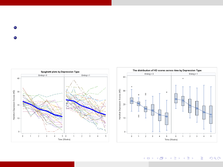
Graphical visualization of Longitudinal Data:
Spaghetti plots (overall, by treatment or other covariates of interest)
Box-plots by time (ove rall, by treatment or other covariates of
interest)
Fares Qeadan, Ph.D (Department of Internal Medicine Division of Epidemiology, Biostatistics, & Preventive MedicineUniversity of New Mexico Health Sciences Center)Longitudinal Data Analysis by Example April 5, 2016 8 / 31
Longitudinal Data Analysis Graphical visualization
Graphical visualization of Longitudinal Data (continued):
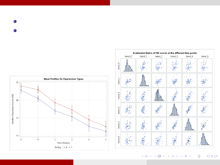
Mean profiles (overall, by treatment or other covariates of interest)
Scatterplot Matrix of the response at the different time points.
Fares Qeadan, Ph.D (Department of Internal Medicine Division of Epidemiology, Biostatistics, & Preventive MedicineUniversity of New Mexico Health Sciences Center)Longitudinal Data Analysis by Example April 5, 2016 9 / 31
Longitudinal Data Analysis Modeling strategies
Modeling strategies:
Traditional Methods:
ANCOVA (adjusting for baseline differences).
Repeated-measures ANOVA (Univariate approach)
MANOVA (Multivariate approach)
Newer Methods:
Generalized Estimating Equations (GEE) Models.
Structural Equations Models.
Transition Models.
Mixed-effects Models
Fares Qeadan, Ph.D (Department of Internal Medicine Division of Epidemiology, Biostatistics, & Preventive MedicineUniversity of New Mexico Health Sciences Center)Longitudinal Data Analysis by Example April 5, 2016 10 / 31
Longitudinal Data Analysis Modeling strategies
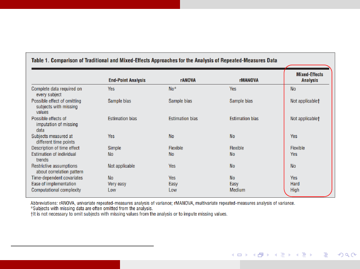
Comparing Mixed-effects Models with Traditional ones
3
:
3
This Table was taken from [9].
Fares Qeadan, Ph.D (Department of Internal Medicine Division of Epidemiology, Biostatistics, & Preventive MedicineUniversity of New Mexico Health Sciences Center)Longitudinal Data Analysis by Example April 5, 2016 11 / 31

Longitudinal Data Analysis Mixed Effects Modeling
Mixed-effects Models [10, 13]:
A mixed model is one that contains both fixed and random effects.
Mixed models for Longitudinal Data explicitly identify individual
(random effects) and population characteristics (fixed effects).
Mixed models are very flexible since they can accommodate any
degree of imbalance in the data.
The mixed effects model has the functional form Y = X β + Z γ +
while the fixed effects model has the functional form Y = X β + .
Assumptions:
The subjects are random sample from the population of interest.
The values of the dependent variable have a multivariate normal
distribution with covariance structure Σ.There are five well known Σ’s
one could assume including: UN, CS, CSH, AR(1)and ARH(1).
Observations from different individuals are independent, while
repeated measureme nts of the same individual are not assumed to be
independent.
If there are missing data, they are assumed to be ignorable (i.e. MAR
or MCAR).
Fares Qeadan, Ph.D (Department of Internal Medicine Division of Epidemiology, Biostatistics, & Preventive MedicineUniversity of New Mexico Health Sciences Center)Longitudinal Data Analysis by Example April 5, 2016 12 / 31

Longitudinal Data Analysis Model selection
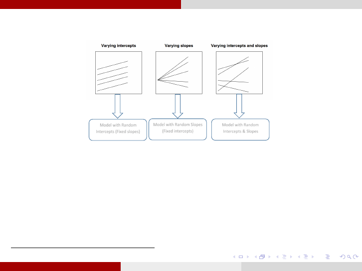
Possible Mixed-effects Models
4
:
Model with Random
Intercepts (Fixed slopes)
Model with Random Slopes
(Fixed intercepts)
Model with Random
Intercepts & Slopes
1. To determine the best covariance structure Σ: use the restricted likelihood ratio
test(G
2
), on the saturated model, with two different covariance structures when the two
structures are nested and AIC or BIC when they are not nested.
2. To determine the best mo del among the above three: use the restricted
likelihood ratio test (G
2
) assuming the selected covariance structure in (1). The three
p ossi ble m ixed-effect models (random intercepts, random slopes, random intercepts &
slopes) are always nested.
4
This Figure is a modification of Figure 11.1 from [11].
Fares Qeadan, Ph.D (Department of Internal Medicine Division of Epidemiology, Biostatistics, & Preventive MedicineUniversity of New Mexico Health Sciences Center)Longitudinal Data Analysis by Example April 5, 2016 13 / 31

Longitudinal Data Analysis Model selection
Possible Mixed-effects Models
4
:
Model with Random
Intercepts (Fixed slopes)
Model with Random Slopes
(Fixed intercepts)
Model with Random
Intercepts & Slopes
1. To determine the best covariance structure Σ: use the restricted likelihood ratio
test(G
2
), on the saturated model, with two different covariance structures when the two
structures are nested and AIC or BIC when they are not nested.
2. To determine the best mo del among the above three: use the restricted
likelihood ratio test (G
2
) assuming the selected covariance structure in (1). The three
p ossi ble m ixed-effect models (random intercepts, random slopes, random intercepts &
slopes) are always nested.
4
This Figure is a modification of Figure 11.1 from [11].
Fares Qeadan, Ph.D (Department of Internal Medicine Division of Epidemiology, Biostatistics, & Preventive MedicineUniversity of New Mexico Health Sciences Center)Longitudinal Data Analysis by Example April 5, 2016 13 / 31

Example: Beating the Blues Background
Example: Beating the Blues
Background [12]:
The data is collected for a clinical trial (Proudfoot et al., 2003)[14].
A new Cognitive-behavioral therapy (CBT) technique called Beating the Blues
(BtB) is tested in a randomized controlled trial of patients suffering from
depression along with treatment as usual (TaU).
The measure used for depression is the Beck Depression Inventory score (BDI) as
describ ed i n Bect et al. (1996)[15].
Measurements were taken on five occasions: prior to treatment, 2, 4, 6, and 8
months later.
Participants of the clinical trial were stratified according to whether they were
prescribed drug or not (yes, no), and the duration of the current episode of
depression (≤ 6 months, ≥ 6 months).
Beating the Blues is a self-help eight-session program that combines computerized
cognitive models with softer science in order to engage the depression patients in a
unique form of therapy. Patients work through modules designed to aid in behavior
modification to help treat different depression symptoms, taking into account
everything from sleeping habits to task breakdown t o problem solving skills.
Fares Qeadan, Ph.D (Department of Internal Medicine Division of Epidemiology, Biostatistics, & Preventive MedicineUniversity of New Mexico Health Sciences Center)Longitudinal Data Analysis by Example April 5, 2016 14 / 31

Example: Beating the Blues Background
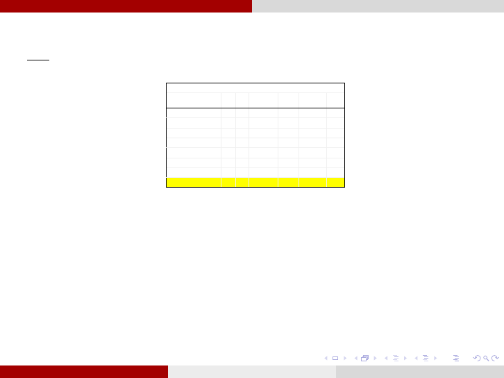
Background (continued):
A recent study published in the British Journal of Psychiatry has recommended
BtB over the general practitioner (GP) treatment as usual for patients in that
country.
Even though BtB has been approved and recognized in the United States by the
National Institute of Health and Clinical Excellence, the effectiveness of its unique
methods is still very much in question by many clinical psychiatrists.
Characteristics of Participants
Total
Beating The
Blues (BtB)
Treatment as
Usual (TaU)
N
%
C.I. (95%)
N
%
C.I. (95%)
N
%
C.I. (95%)
Total
100
100%
NA
52
52%
(42.0-62.0)
48
48%
(38.0-58.0)
Prescribed
Drug
Yes
44
44%
(34.1-53.9)
30
30%
(20.9-39.1)
14
14%
(7.1-20.9)
No
56
56%
(46.1-65.9)
22
22%
(13.7-30.3)
34
34%
(24.5-43.4)
Length of
Illness
Less Than 6 months
49
49%
(39.0-59.0)
26
26%
(17.2-34.7)
23
23%
(14.6-31.4)
>=6m
51
51%
(41.0-61.0)
26
26%
(17.2-34.7)
25
25%
(16.4-33.6)
Remark 3.All analyses in this work were done using the PROC MIXED procedure in
SAS.
Remark 4.Data was obtained from [16].
Fares Qeadan, Ph.D (Department of Internal Medicine Division of Epidemiology, Biostatistics, & Preventive MedicineUniversity of New Mexico Health Sciences Center)Longitudinal Data Analysis by Example April 5, 2016 15 / 31

Example: Beating the Blues Background
Background (continued):
A recent study published in the British Journal of Psychiatry has recommended
BtB over the general practitioner (GP) treatment as usual for patients in that
country.
Even though BtB has been approved and recognized in the United States by the
National Institute of Health and Clinical Excellence, the effectiveness of its unique
methods is still very much in question by many clinical psychiatrists.
Characteristics of Participants
Total
Beating The
Blues (BtB)
Treatment as
Usual (TaU)
N
%
C.I. (95%)
N
%
C.I. (95%)
N
%
C.I. (95%)
Total
100
100%
NA
52
52%
(42.0-62.0)
48
48%
(38.0-58.0)
Prescribed
Drug
Yes
44
44%
(34.1-53.9)
30
30%
(20.9-39.1)
14
14%
(7.1-20.9)
No
56
56%
(46.1-65.9)
22
22%
(13.7-30.3)
34
34%
(24.5-43.4)
Length of
Illness
Less Than 6 months
49
49%
(39.0-59.0)
26
26%
(17.2-34.7)
23
23%
(14.6-31.4)
>=6m
51
51%
(41.0-61.0)
26
26%
(17.2-34.7)
25
25%
(16.4-33.6)
Remark 3.All analyses in this work were done using the PROC MIXED procedure in
SAS.
Remark 4.Data was obtained from [16].
Fares Qeadan, Ph.D (Department of Internal Medicine Division of Epidemiology, Biostatistics, & Preventive MedicineUniversity of New Mexico Health Sciences Center)Longitudinal Data Analysis by Example April 5, 2016 15 / 31

Example: Beating the Blues Research Questions
Objectives:
To assess the effectiveness of the BtB as a mode of delivery of
Cognitive-behavioral therapy. To do so, we examine the following research
questions:
1
Do BtB and TaU differ in their effects on depression?
2
Do the patterns of change over time differ in the two treatment
groups? Does one treatment show results more quickly?
3
Do the effects of BtB (and TaU) differ in patients who did or did not
receive the drugs?
4
Do the patterns of change over time differ in the BtB (and TaU)
group by drug therapy?
5
Do the patterns of change over time differ in the BtB (and TaU)
group by length of illness and drug therapy?
Fares Qeadan, Ph.D (Department of Internal Medicine Division of Epidemiology, Biostatistics, & Preventive MedicineUniversity of New Mexico Health Sciences Center)Longitudinal Data Analysis by Example April 5, 2016 16 / 31
Example: Beating the Blues Selecting the Covariance Structure
Selecting the Covariance Structure: To select the covariance structure, we
compare the saturated model with different covariance patterns. The saturated model
includes all covariate variables as well as the corresponding interaction terms:
(1)
lengthmonthdrugmonthmonthlengthdruglengthdrugBDIE ***)(
lengthtreatmentdrugtreatmenttreatmentlengthdrugmonth ****
drugtreatmentmonthtreatmentmonthlengthdrugtreatment *****
lengthdrugtreatmentmonthlengthtreatmentmonth *****
Covariance Pattern Model
-2(REML) Log-Likelihood
AIC
UN (15 parameters)
2428.8
2458.8
CS (2 parameters)
2461.8
2465.8
CSH (6 parameters)
2457.2
2469.2
AR(1) (2 parameters)
2462.8
2466.8
ARH(1) (6 parameters)
2454.2
2466.2
Table 1: Covariance Pattern Model
Covariance models
G^2
(nested)
Df
(nested)
p-value
(nested)
Best model
(nested)
Lowest AIC
(non-nested)
UN vs. CS
33
15-2=13
0.001704
UN
UN vs. CSH
28.4
15-6=9
0.0008176
UN
UN vs. AR(1)
34
15-2=13
0.0012036
UN
UN vs. ARH(1)
25.4
15-6=9
0.0025591
UN
CS vs. CSH
4.6
6-2=4
0.3308542
CS
CS vs. AR(1)
CS
CS vs. ARH(1)
CS
CSH vs. AR(1)
AR(1)
CSH vs. ARH(1)
ARH(1)
AR(1) vs. ARH(1)
8.6
6-2=4
0.0719134
AR(1)
Table 2: Covariance Models’ Comparisons
The unstructured covariance model was found to be most adequate.
Fares Qeadan, Ph.D (Department of Internal Medicine Division of Epidemiology, Biostatistics, & Preventive MedicineUniversity of New Mexico Health Sciences Center)Longitudinal Data Analysis by Example April 5, 2016 17 / 31
Example: Beating the Blues Analysis for Research Questions
1. Do BtB and TaU differ in their effects on depression?
Model:
treatmentmonthlengthdrugBDIE )(
Type 3 Tests of Fixed Effects
Effect
Num
DF
Den
DF
Chi-Square
F Value
Pr > ChiSq
Pr > F
Drug
1
279
1.07
1.07
0.3012
0.3021
Length
1
279
3.46
3.46
0.0630
0.0641
month
1
279
115.16
115.16
<.0001
<.0001
Treatment
1
279
4.83
4.83
0.0280
0.0288
1. We will favor the model with random varying
intercepts (p-value=0.142) and without
interaction effect (model selection p-
value=0.403).
2. So, there is strong evidence (p-value=0.029) to
suggest that BtB and TaU differ in their effects
on depression, as reflected by the BDI score.
Remark 5.Null and alternative hypotheses for model selection:
H
0
: Model with random intercepts is adequate
H
1
: Model with random intercepts and slopes is adequate
H
0
: Model without interaction is adequate
H
1
: Model with interaction is adequate
Fares Qeadan, Ph.D (Department of Internal Medicine Division of Epidemiology, Biostatistics, & Preventive MedicineUniversity of New Mexico Health Sciences Center)Longitudinal Data Analysis by Example April 5, 2016 18 / 31
Example: Beating the Blues Analysis for Research Questions
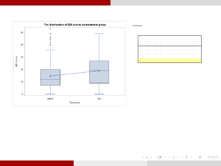
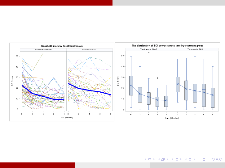
2. Do the patterns of change over time differ in the two treatment
groups? Does one treatment show results more quickly?
Remark 6.We observe a decreasing variance across time for the BtB treatment but not
for the TaU.
Remark 7.We observe a general linear decline over time for both treatments.
Fares Qeadan, Ph.D (Department of Internal Medicine Division of Epidemiology, Biostatistics, & Preventive MedicineUniversity of New Mexico Health Sciences Center)Longitudinal Data Analysis by Example April 5, 2016 19 / 31
Example: Beating the Blues Analysis for Research Questions
(continued)
Model:
monthtreatmenttreatmentmonthl engthdrugBDIE *)(
Type 3 Tests of Fixed Effects
Effect
Num
DF
Den
DF
Chi-Square
F Value
Pr > ChiSq
Pr > F
Drug
1
278
1.03
1.03
0.3101
0.3110
Length
1
278
3.22
3.22
0.0726
0.0737
month
1
278
113.67
113.67
<.0001
<.0001
Treatment
1
278
3.04
3.04
0.0812
0.0823
month*Treatment
1
278
0.67
0.67
0.4119
0.4126
1. We will favor the model with random varying
intercepts (p =0.135). Even though a model without
interaction effect is more adequate (model selection p
=0.403) we will include the interaction term to
examine this particular research question.
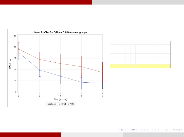
2. So, there is no evidence of difference (p =0.413) in the
pattern of change of BDI score between subjects
receiving BtB and TaU over time. Even though the BDI
score mean plot reveals that BtB shows results more
quickly than TaU, there is no statistical significance to
infer such a thing.
Fares Qeadan, Ph.D (Department of Internal Medicine Division of Epidemiology, Biostatistics, & Preventive MedicineUniversity of New Mexico Health Sciences Center)Longitudinal Data Analysis by Example April 5, 2016 20 / 31
Example: Beating the Blues Analysis for Research Questions
3. Do the effects of BtB (and TaU) differ in patients who did or did
not receive the drugs?
Model:
drugtreatmenttreatmentmonthlengthdrugBDIE *)(
Type 3 Tests of Fixed Effects
Effect
Num
DF
Den
DF
Chi-Square
F Value
Pr > ChiSq
Pr > F
Drug
1
279
0.83
0.83
0.3622
0.3630
Length
1
279
3.32
3.32
0.0683
0.0693
month
1
279
114.34
114.34
<.0001
<.0001
Treatment
1
279
3.96
3.96
0.0467
0.0477
Treatment*Drug
1
279
0.57
0.57
0.4519
0.4526
1. We will favor the model with random varying intercepts (p
=0.165). Even though a model without interaction effect is
more adequate (model selection p =0.741) we will include
the interaction term to examine this particular research
question.
2. So, there is no evidence (p =0.453) that the effect of BtB (or
TaU) is different in patients who did or did not receive drug.
However, the pattern of change of BtB (or TaU) effect is
different in patients who did or did not receive drug as
illustrated in the next research question (p-value=0.0508)
Fares Qeadan, Ph.D (Department of Internal Medicine Division of Epidemiology, Biostatistics, & Preventive MedicineUniversity of New Mexico Health Sciences Center)Longitudinal Data Analysis by Example April 5, 2016 21 / 31
Example: Beating the Blues Analysis for Research Questions
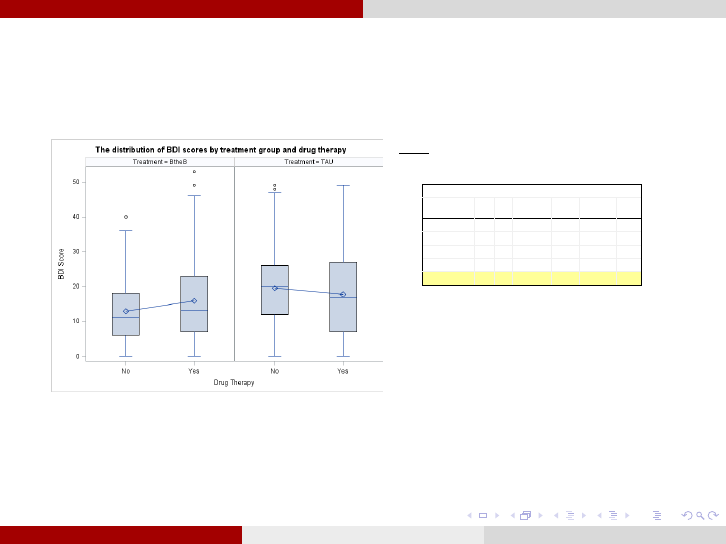
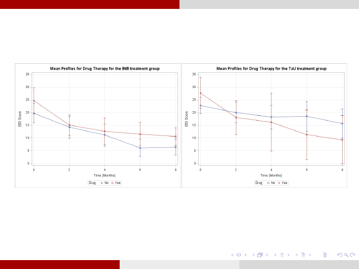
4. Do the patterns of change over time differ in the BtB (and TaU)
group by drug therapy?
Remark 8.We observe a positive effect between Drug Therapy and TaU treatment
(b eing in Drug therapy with TaU treatment gives lower mean BDI scores).
Remark 9.We observe a negative effect between Drug Therapy and BtB treatment
(b eing in Drug therapy with BtB treatment gives higher mean BDI scores).
Fares Qeadan, Ph.D (Department of Internal Medicine Division of Epidemiology, Biostatistics, & Preventive MedicineUniversity of New Mexico Health Sciences Center)Longitudinal Data Analysis by Example April 5, 2016 22 / 31
Example: Beating the Blues Analysis for Research Questions
(continued)
Model:
drugtreatmentmonthtreatmentmonthdrugmonthdrugtreatmenttreatmentmonthlengthdrugBDIE *****)(
Type 3 Tests of Fixed Effects
Effect
Num
DF
Den
DF
Chi-Square
F Value
Pr > ChiSq
Pr > F
Drug
1
276
2.70
2.70
0.1003
0.1015
Length
1
276
3.50
3.50
0.0614
0.0624
month
1
276
121.06
121.06
<.0001
<.0001
Treatment
1
276
3.60
3.60
0.0579
0.0590
Treatment*Drug
1
276
0.00
0.00
0.9909
0.9909
month*Drug
1
276
4.84
4.84
0.0279
0.0287
month*Treatment
1
276
0.00
0.00
0.9688
0.9688
month*Treatment*Drug
1
276
3.85
3.85
0.0498
0.0508
1. We will favor the model with random varying intercepts (p =0.407). A model with 3-way interaction effect is more adequate (model selection
p =0.0134).
2. So, at the 10% significance level, there is evidence (p =0.0508) that the pattern of change of BtB (or TaU) effect is different in patients who did
or did not receive drug.
Remark 10.The use of BtB treatment in CBT brings significant clinical improvement in
anxiety and depression as compared to TaU. While there was no interaction of BtB with
Drug therapy over time, there was an interaction of TaU with Drug therapy, which was
found to be marginally statistically significant (p=0.0508). This indicates that TaU
brings about a feeling of relaxation more swiftly in patients receiving Drug therapy than
those who are not. Note that this result was ignored by Proudfo ot.
Fares Qeadan, Ph.D (Department of Internal Medicine Division of Epidemiology, Biostatistics, & Preventive MedicineUniversity of New Mexico Health Sciences Center)Longitudinal Data Analysis by Example April 5, 2016 23 / 31
Example: Beating the Blues Analysis for Research Questions
5. Do the patterns of change over time differ in the BtB (and TaU)
group by length of illness and drug therapy?
Model:
treatmentmonthlengthdrugBDIE |||)(
Type 3 Tests of Fixed Effects
Effect
Num
DF
Den
DF
Chi-Square
F Value
Pr > ChiSq
Pr > F
Drug
1
272
2.58
2.58
0.1081
0.1092
Length
1
272
3.00
3.00
0.0831
0.0843
Drug*Length
1
272
0.88
0.88
0.3485
0.3493
month
1
272
119.95
119.95
<.0001
<.0001
month*Drug
1
272
3.67
3.67
0.0553
0.0564
month*Length
1
272
0.03
0.03
0.8722
0.8723
month*Drug*Length
1
272
1.33
1.33
0.2484
0.2495
Treatment
1
272
3.69
3.69
0.0546
0.0557
Treatment*Drug
1
272
0.00
0.00
0.9603
0.9603
Treatment*Length
1
272
0.18
0.18
0.6683
0.6686
Treatmen*Drug*Length
1
272
0.23
0.23
0.6307
0.6311
month*Treatment
1
272
0.07
0.07
0.7982
0.7984
month*Treatment*Drug
1
272
2.87
2.87
0.0903
0.0914
month*Treatme*Length
1
272
0.75
0.75
0.3878
0.3885
mont*Trea*Drug*Lengt
1
272
0.82
0.82
0.3644
0.3652
1. We will favor the model with random varying intercepts (p =0.472). A model with 4-way interaction effect is adequate (model
selection p =0.0003).
2. Results from this model should be interpreted with cautions due to the possibility of over-fitting.
Fares Qeadan, Ph.D (Department of Internal Medicine Division of Epidemiology, Biostatistics, & Preventive MedicineUniversity of New Mexico Health Sciences Center)Longitudinal Data Analysis by Example April 5, 2016 24 / 31
Example: Beating the Blues Pitfalls
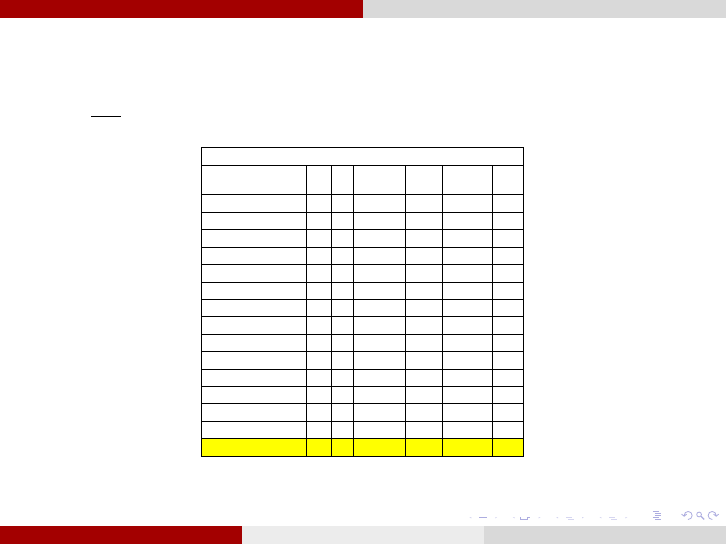
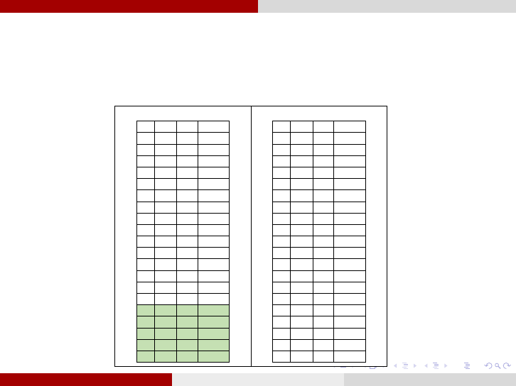
High Order Interaction Terms:To make a reliable statistical inference from
comp ound i nteraction terms, the sample size of the subgroups due interaction must be
reasonably large. Separati on tables could be used for this purpose such that cell sizes
less than 10 are usually an indication for poor results and possible over-fitting.
TaU treatment group:
Drug
Length
month
Frequency
No
<6m
0
15
No
<6m
2
15
No
<6m
4
15
No
<6m
6
15
No
<6m
8
15
No
>6m
0
19
No
>6m
2
19
No
>6m
4
19
No
>6m
6
19
No
>6m
8
19
Yes
<6m
0
8
Yes
<6m
2
8
Yes
<6m
4
8
Yes
<6m
6
8
Yes
<6m
8
8
Yes
>6m
0
6
Yes
>6m
2
6
Yes
>6m
4
6
Yes
>6m
6
6
Yes
>6m
8
6
BtB treatment group:
Drug
Length
month
Frequency
No
<6m
0
9
No
<6m
2
9
No
<6m
4
9
No
<6m
6
9
No
<6m
8
9
No
>6m
0
13
No
>6m
2
13
No
>6m
4
13
No
>6m
6
13
No
>6m
8
13
Yes
<6m
0
17
Yes
<6m
2
17
Yes
<6m
4
17
Yes
<6m
6
17
Yes
<6m
8
17
Yes
>6m
0
13
Yes
>6m
2
13
Yes
>6m
4
13
Yes
>6m
6
13
Yes
>6m
8
13
Fares Qeadan, Ph.D (Department of Internal Medicine Division of Epidemiology, Biostatistics, & Preventive MedicineUniversity of New Mexico Health Sciences Center)Longitudinal Data Analysis by Example April 5, 2016 25 / 31

Example: Beating the Blues Inference on Individuals
Inference on Individuals versus Population:
Model for the population (the intercept is the same for all individuals):
treatmentmonthlengthdrugE
BDI
i
43210
treatmentmonthlengthdrugE
BDI
i
32.436.152.307.222.21
Model for the individuals (the intercept differs from individual to another):
treatmentmonthlengthdrugE
i
i
BDI
432100
treatmentmonthlengthdrugE
i
i
BDI
32.436.152.307.222.21
0
Fares Qeadan, Ph.D (Department of Internal Medicine Division of Epidemiology, Biostatistics, & Preventive MedicineUniversity of New Mexico Health Sciences Center)Longitudinal Data Analysis by Example April 5, 2016 26 / 31

References
References
[1]. Van Belle, G., Fisher, L. D., Heagerty, P. J., & Lumley, T. (2004).
Biostatistics: a methodology for the health sciences (Vol. 519). John
Wiley & Sons.
[2]. Molenaar, P. C. (1997). Time series analysis and its relationship
with longitudinal analysis. International Journal of sports medicine, 18,
S232-7.
[3]. Riesby, N. et al.( 1977). Imipramine: Clinical effects and
pharmacokinetic variability. Psychopharmacology, 54,263-272.
[4]. Christopher Slayden and Julie Riley. Seasonal Variance in the
Presentation of Urolithiasis [GME Project], March, 2016. University of
New Mexico Health Sciences Center.
[5]. Twisk, J. W. (2013). Applied longitudinal data analysis for
epidemiology: a practical guide. Cambridge University Press.
Fares Qeadan, Ph.D (Department of Internal Medicine Division of Epidemiology, Biostatistics, & Preventive MedicineUniversity of New Mexico Health Sciences Center)Longitudinal Data Analysis by Example April 5, 2016 27 / 31

References
[6]. Liu, X. (2015). Methods and Applications of Longitudinal Data
Analysis. Elsevier.
[7]. Fitzmaurice, G. M., Laird, N. M., & Ware, J. H. (2012). Applied
longitudinal analysis (Vol. 998). John Wiley & Sons.
[8]. Hedeker, D., & Gibbons, R. D. (2006). Longitudinal data analysis
(Vol. 451). John Wiley & Sons.
[9]. Ralitza Gueorguieva, PhD; John H. Krystal, MD Move Over
ANOVA : Progress in Analyzing Repeated-Measures Data and Its
Reflection in Papers Published in the Archives of General Psychiatry.
Arch Gen Psychiatry.2004;61:310-317.
[10]. Garrett M. Fitzmaurice. Lecture Notes on Longitudinal Data
Analysis. Harvard T.H. Chan School of Public Health:(March, 27,
2016) http://www.hsph.harvard.edu/fitzmaur/ala/lectures.p df
[11]. Gelman, A., & Hill, J. (2006). Data analysis using regression and
multilevelhierarchical models. Cambridge University Press.
Fares Qeadan, Ph.D (Department of Internal Medicine Division of Epidemiology, Biostatistics, & Preventive MedicineUniversity of New Mexico Health Sciences Center)Longitudinal Data Analysis by Example April 5, 2016 28 / 31

References
[12]. Fares Qeadan & Brianna Killian (May, 2007). BtB: An Analysis
of a Cognitive Behavioral Therapy Technique used in Treating
Depression. Final project for STAT 775 (Dr. DoHwan Park).
[13] Ronald Christense (2001). Advanced Linear Modeling. Springer.
[14] Proudfoot, J., Goldberg, D., Mann, A., Everitt, B., Marks, I., &
Gray, J. A. (2003). Computerized, interactive, multimedia
cognitive-behavioural program for anxiety and depression in general
practice. Psychological medicine, 33(02), 217-227.
[15] Beck, A. T., Steer, R. A., Ball, R., & Ranieri, W. F. (1996).
Comparison of Beck Depression Inventories-IA and-II in psychiatric
outpatients. Journal of personality assessment, 67(3), 588-597.
[16] Everitt, B. S. (2006). An R and S-PLUS companion to
multivariate analysis. Springer Science & Business Media. Chicago
Fares Qeadan, Ph.D (Department of Internal Medicine Division of Epidemiology, Biostatistics, & Preventive MedicineUniversity of New Mexico Health Sciences Center)Longitudinal Data Analysis by Example April 5, 2016 29 / 31


Citation
How to cite this work:
This work was funded by the NIH grants (1U54GM104944-01A1) through the
National Institute of General Medical Sciences (NIGMS) under the Institutional
Development Award (IDeA) program and the UNM Clinical & Translational
Science Center (CTSC) grant (UL1TR001449). Thus, to cite this work please
use:
Fares Qeadan (2016). Longitudinal Data Analysis by Example. A seminar
in biostatistics for the Mountain West Clinical Translational Research
Infrastructure Network (grant 1U54GM104944) and UNM Clinical &
Translational Science Center (CTSC) (gran t UL1TR001449). University of
New Mexico Health Sciences Center. Albuquerque, New Mexico.
Fares Qeadan, Ph.D (Department of Internal Medicine Division of Epidemiology, Biostatistics, & Preventive MedicineUniversity of New Mexico Health Sciences Center)Longitudinal Data Analysis by Example April 5, 2016 31 / 31
