Page 1
C
C
o
o
u
u
r
r
s
s
e
e
T
T
o
o
p
p
i
i
c
c
s
s
:
:
I. Microsoft Excel Overview
II. Navigating Spreadsheets in Excel
III. Entering and Editing Data
IV. Using Formulas and Functions
V. Sorting and Filtering Data
VI. Applying a Custom AutoFilter
Section 1 – Overview
W
W
h
h
a
a
t
t
i
i
s
s
M
M
i
i
c
c
r
r
o
o
s
s
o
o
f
f
t
t
E
E
x
x
c
c
e
e
l
l
?
?
Microsoft Excel is a spreadsheet program, which means that it is primarily
used to create and edit numbers and text in cells. A cell is the intersection
of a column and a row and can contain an unlimited amount of characters.
A spreadsheet used to be a large sheet of grid-lined paper that spread
across a desk; it was used in accounting to keep columns of numbers lined
up. When computerized spreadsheets were developed, this grid structure
was kept intact.
Computerized spreadsheets have many advantages over the old paper
spreadsheets. Formatting is much easier, and Excel can perform calculations
on spreadsheet data that would be impossible on a paper sheet!
Spreadsheets are contained in a file called a workbook. Microsoft Excel
includes many helpful features to enhance the text and layout of
spreadsheets.
O
O
v
v
e
e
r
r
v
v
i
i
e
e
w
w
o
o
f
f
E
E
x
x
e
e
r
r
c
c
i
i
s
s
e
e
s
s
f
f
o
o
r
r
L
L
e
e
v
v
e
e
l
l
1
1
1. Start Microsoft Excel (Start > All Programs > Microsoft Office >
Microsoft Office Excel 2003). A blank workbook called “Book1”
automatically opens. Look over the interface. Click the smaller Close
Window button to close it.
2. Open the file called “IntroDone.xls” (File > Open > Desktop >
Training > Excel).
3. Scroll through the spreadsheet, noting the major features to be
discussed in Level 1.
Excel 2003, Level 1 Page 2
September 2005
Section 2 – Navigating Spreadsheets in Excel
U
U
s
s
i
i
n
n
g
g
C
C
o
o
l
l
u
u
m
m
n
n
s
s
a
a
n
n
d
d
R
R
o
o
w
w
s
s
Data are entered in columns (vertical) and rows (horizontal). Columns are
lettered A-Z (then AA-AZ, BA-BZ, and so on, through column IV). Rows
are numbered. There are 256 columns and 65,536 rows in every
spreadsheet. That’s a total of more than 16 million cells per sheet! A cell
is the intersection of a column and a row. (Example, cell A1 is at the
intersection of column A, row 1.)
S
S
c
c
r
r
o
o
l
l
l
l
i
i
n
n
g
g
T
T
h
h
r
r
o
o
u
u
g
g
h
h
t
t
h
h
e
e
S
S
p
p
r
r
e
e
a
a
d
d
s
s
h
h
e
e
e
e
t
t
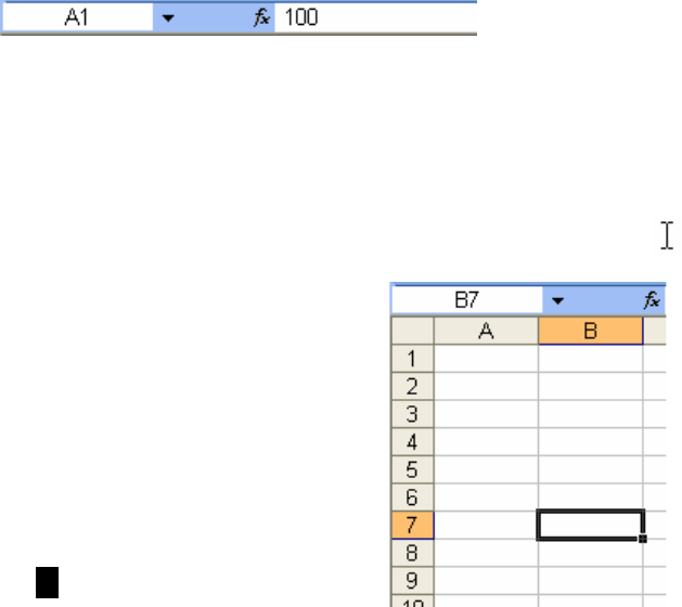
Clicking on a cell selects that cell. When a cell is selected, the Name Box
indicates which cell is active, and the formula bar displays the contents of
that cell. Note that the formula may be different than what is displaying in
the cell when you look at the spreadsheet.
name box formula bar
Entering and editing text is accomplished by double-clicking the mouse
pointer over the desired place and clicking a fine area in the cell called the
“insertion point.” This is the point at which text will begin to be entered, a
selection will begin, or a graphic or other file will be inserted. The mouse
arrow changes to a text selection pointer called the “I-Beam” pointer.
1. Open the file called
“Introduction.xls” Click on cell B7.
The Name Box indicates that B7 is the
active cell. Click in another location,
and the Name Box changes.
2. To select multiple cells, click in the
middle of on cell, then drag-select the
desired range of cells using the large
white cross pointer (®).
3. Scroll using the scroll bar arrows on the right side of the screen. Note
that as you scroll, the active cell does not change. Also try scrolling by
clicking above or below the scroll button, as well as dragging and
dropping the scroll button itself. Use the horizontal scroll bar to view
additional columns; use the vertical scroll bar to view additional rows.
Excel 2003, Level 1 Page 3
September 2005
4. Several ways to select cells without using the mouse:
a. Press the arrow keys on the keyboard to scroll one row at a time (up
or down), or one column at a time (right or left).
b. The enter key moves down one cell, the tab key moves to the right.
c. Also use the Page Up and Page Down keys, above the arrow keys.
d. Press the Home key to move to the beginning of a row.
e. Press the End key then any arrow key to move to the next major row
or column group which contains data.
f. Press Ctrl+Home to jump to the first active cell in the spreadsheet.
g. Press Ctrl+End to jump to the last active cell in the spreadsheet.
Note that all keyboard movements change the active cell.
C
C
h
h
a
a
n
n
g
g
i
i
n
n
g
g
t
t
h
h
e
e
Z
Z
o
o
o
o
m
m
D
D
i
i
s
s
p
p
l
l
a
a
y
y
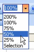
Use the Zoom Box to change the magnification of the data on the screen.
The Zoom Box only changes the view of what is on the screen; it does not
change the printed worksheet or active cell.
1. Select Sheet 2 then click the down arrow
next to the Zoom Box and select 50%.
The spreadsheet zooms out.
2. Click again on the down arrow and
change the zoom to 200%.
The spreadsheet zooms in on the active cell.
3. Click inside the Zoom Box, type an amount of 73, then press Enter.
The spreadsheet zooms to a custom zoom of 73%.
4. Reset the zoom to 100% to return the spreadsheet to its original size.
Excel 2003, Level 1 Page 4
September 2005
N
N
a
a
v
v
i
i
g
g
a
a
t
t
i
i
n
n
g
g
t
t
o
o
O
O
t
t
h
h
e
e
r
r
W
W
o
o
r
r
k
k
s
s
h
h
e
e
e
e
t
t
s
s
A workbook can contain an unlimited number of worksheets. The default
number of worksheets in a new workbook is 3. (The default can be changed
under Tools > Options > General)
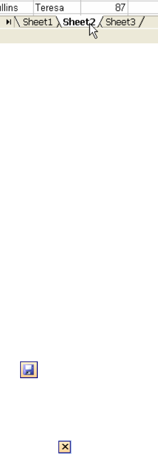
1. Click the Sheet2 tab at the
bottom of the window.
Sheet2 displays, with cell A1
active. Click on cell B8.
2. Click the Sheet3 tab.
Sheet3 displays, with cell A1 active.
3. Click on the Sheet2 tab. Note that cell B8 is still the active cell.
4. Click on the Sheet1 tab. Note that the last active cell is still active. Excel
tracks the active cell in each worksheet until the workbook is closed, at
which time all sheets return to the active cell when the workbook was last
saved.
D
D
e
e
l
l
e
e
t
t
i
i
n
n
g
g
S
S
h
h
e
e
e
e
t
t
s
s
1. Right-click the Sheet3 sheet tab and choose Delete.
If the worksheet contains any data, a dialog box displays warning
that the entire sheet and all its data will be permanently deleted.
2. Click Delete to delete the sheet.
3. Return to Sheet1 and Save (File > Save or
) the file.
C
C
l
l
o
o
s
s
i
i
n
n
g
g
a
a
W
W
o
o
r
r
k
k
b
b
o
o
o
o
k
k
Click the workbook’s close window button (the lower
icon) to close it (Or
choose File > Close). Close all open workbooks. The screen shows a blank,
gray application screen.
Excel 2003, Level 1 Page 5
September 2005
Section 3 – Entering and Editing Data
E
E
n
n
t
t
e
e
r
r
i
i
n
n
g
g
D
D
a
a
t
t
a
a
i
i
n
n
a
a
B
B
l
l
a
a
n
n
k
k
W
W
o
o
r
r
k
k
s
s
h
h
e
e
e
e
t
t
1. Open the file called “Introduction.xls”. We will create a simple Budget
Spreadsheet using a blank worksheet in Excel.
2. Ensure that Sheet1 is blank and that Sheet2 has student names and
grades. Return to Sheet 1.
3. Type “Cash on Hand” in cell A3 and press Enter.
4. Type “Paycheck” in cell A4 and press Enter.
(The number pad’s Enter also works.)
5. Type “Total” in cell A5 and click on cell B3.
6. Type “500” in cell B3 and press Enter (can use the number pad.)
7. Type “500” in cell B4 and press Enter (can use the number pad.)
Note that some wording “spills over” to an adjacent cell.
as you type. The width of a column can be adjusted to
accommodate the text in cells.
NOTE: By default text is left aligned, and numbers are right
aligned.
Excel 2003, Level 1 Page 6
September 2005
U
U
s
s
i
i
n
n
g
g
S
S
h
h
o
o
r
r
t
t
c
c
u
u
t
t
s
s
W
W
h
h
e
e
n
n
E
E
n
n
t
t
e
e
r
r
i
i
n
n
g
g
D
D
a
a
t
t
a
a
1. When entering data across the columns, press the right arrow key
instead of Enter to move to the next column. Use the other arrow keys
to move in any other desired direction.
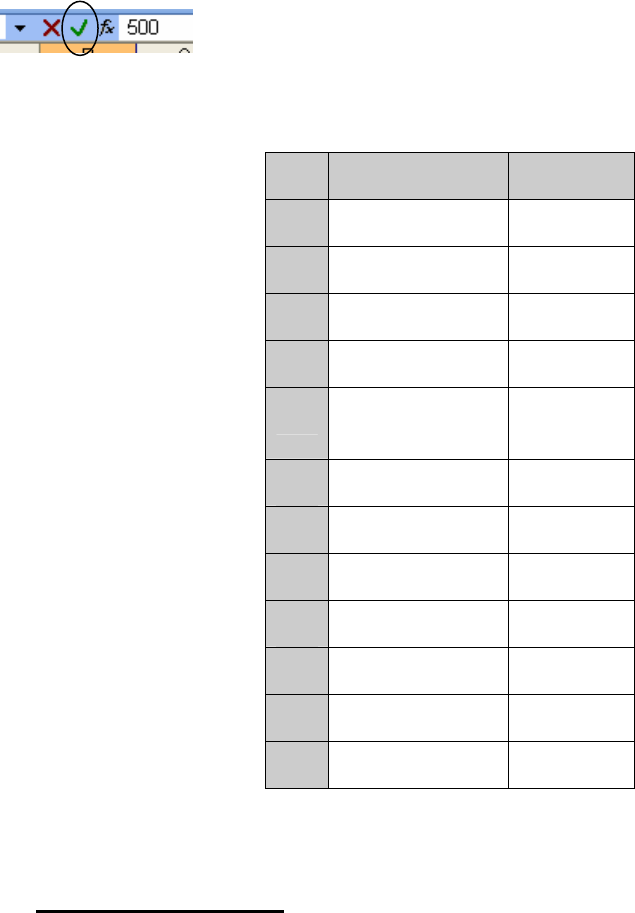
2. To accept the entry in a cell without moving the active cell, or “cell
designator”, click the green check mark next to the Edit Line on the
Formula Bar (it is active only as you enter data in the cell).
(X) is cancel, (
a
) is enter/accept, and (fx) is edit formula.
3. Continue to enter the rest of the data, as shown below:
A B
7
Phone 80
8
Electric 75
9
Cable 25
10
Utilities Total
11
Average
Utility
12
13
Utilities Total
14
Auto 250
15
Rent 350
16
Total
17
Money Left
18
E
E
d
d
i
i
t
t
i
i
n
n
g
g
T
T
e
e
x
x
t
t
1.
Directly in the Cell
a. Click on cell C2, type your first name, and click the green check
mark next to the Edit Line to accept the contents without moving to a
new cell.

Excel 2003, Level 1 Page 7
September 2005
b. Click on cell D2, type your last name, and press Enter.
c. Select cell D2 and press the Delete key, or Edit > Undo on the menu
bar. (If you had not pressed Enter, the Escape Key would undo.)
The cell’s contents are deleted and cleared to a blank cell.
d. Select cell C2 and begin typing your campus phone number. The new
entry wipes out the old entry. Before you finish, click the red “X” next to
the Edit Line. (This does the same thing as the Esc key.)
The cell’s contents are returned to the previous entry.
e. Delete cell C2 by either pressing the Backspace or the Delete key.
2.
Using the Edit Line
If a cell’s contents are already mostly correct, it is not necessary to wipe
out the entire cell and re-type the contents. You can use the Edit Line to
make minor adjustments to cells.
a. Select cell A11 (Average Utility).
b. In the Edit Line, click to the right of the “y” in “Utility”, press
Backspace, then type “ies” to make it read “Utilities”.
c. Press Enter (or the green check mark) to accept the change.
W
W
i
i
d
d
e
e
n
n
i
i
n
n
g
g
C
C
o
o
l
l
u
u
m
m
n
n
s
s
1.
By Dragging
a. Place the mouse pointer between the column A and column B headings
at the top of the window.
The pointer changes to a double-headed horizontal arrow.
b. Click-and-drag the column heading line until the width pop-up box
above the pointer reads “24.00”. This is the number of characters that
can be contained in a column of that width. Release the mouse button to
accept the width of 24.00.

Excel 2003, Level 1 Page 8
September 2005
2.
By Using AutoFit
AutoFit is a feature that automatically sizes a column to fit the longest string
of text in that column. To use AutoFit, simply double-click the line between
column headings after the cursor changes to the double-headed
horizontal arrow. There are two important notes about using AutoFit:
a. AutoFit does not adjust columns if any additional text is typed into the
column after you applied it. If additional text does not fit in the current
column width, you must AutoFit again to adjust to the new text.
b. Sometimes, you do not want to size a column according to the longest
item in it. If AutoFit results in a column wider than you actually intended,
manually resize the column to your own preference.
I
I
n
n
s
s
e
e
r
r
t
t
i
i
n
n
g
g
/
/
D
D
e
e
l
l
e
e
t
t
i
i
n
n
g
g
R
R
o
o
w
w
s
s
To properly space out the “Money Left” row from the others,
1. Click on cell A17 (Money Left).
2. Choose Insert > Rows to insert a new blank row (17) above, and
“Money Left” moves down to row 18.
3. Delete a row, column or cell by selecting it and choosing Edit > Delete.
NOTE: Inserting Rows/Columns does not destroy any active formulas!
R
R
e
e
n
n
a
a
m
m
i
i
n
n
g
g
W
W
o
o
r
r
k
k
s
s
h
h
e
e
e
e
t
t
s
s
1.
By Right-Clicking
a. Right-click the Sheet1 sheet tab and choose Rename.
The current name is highlighted.
b. Type “Checkbook” and press Enter to accept the new name.
2.
By Double-Clicking
a. Double-click the Sheet2 sheet tab. The name is now highlighted.
b. Type “Grades” and press Enter, and Save the workbook.
Excel 2003, Level 1 Page 9
September 2005
Section 4 – Using Formulas and Functions
W
W
h
h
a
a
t
t
i
i
s
s
a
a
F
F
o
o
r
r
m
m
u
u
l
l
a
a
?
?
A formula is a calculated (or “derived”) field used by Excel in the place of
typed entries. To see the reasons for using formulas, try to complete the
checkbook in the following manner:
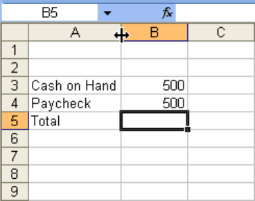
1. Click on cell B5. Add the figures together in cells B3 and B4, then type
the result (1000) in cell B5.
2. Ooops! The “Cash on Hand” figure should actually be 400, not 500 as
currently shown. Change the amount in cell B3 to “400”.
3. Note that the figure in cell B5 does not change, even though it is now
incorrect. To correct this cell, you would have to manually change it as
well. Other changes would have to be made throughout the spreadsheet,
such as to cell B18 (Money Left), when completed.
4. Delete the entry in cell B5. Change the amount in cell B3 to “500”.
E
E
n
n
t
t
e
e
r
r
i
i
n
n
g
g
a
a
F
F
o
o
r
r
m
m
u
u
l
l
a
a
What you actually intend in cell B5 is to add together the amounts in cells B3
and B4 and display the result, while allowing for future changes. This
process is called using a cell reference to prepare a formula. A cell
reference can refer to one or more cells.
IMPORTANT: You must enter an equal sign (
=) to begin a formula. You
must follow the rules of the “order of operations” when writing formula:
“(3 + 1)/2” is not the same as “3 + 1 / 2”
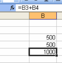
1. In cell B5, type “=B3+B4” and press Enter. (You
do not have to type capital letters; Excel will
automatically convert cell references for you.)
The resulting calculation of 1000 displays in
the cell.
2. Click back on cell B5 and view the contents of the
Edit Line. The formula, not the number “1000”, is
shown.
3. Click on cell B3 and type “600”.
Excel 2003, Level 1 Page 10
September 2005
Cell B5 automatically updates to 1100.
Q: Why didn’t we
use the formula
“=500+500”?
T
T
y
y
p
p
i
i
n
n
g
g
a
a
C
C
e
e
l
l
l
l
R
R
a
a
n
n
g
g
e
e
A range is a group of two or more adjacent cells. Ranges are entered in this
way: “B7:B9”. The colon is a mathematical substitute for the word
“through” in a formula. Ranges are often used in coordination with
functions (sum, average, count, etc.).
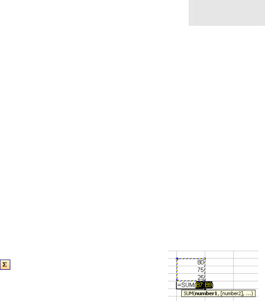
1. Click on cell B10.
2. Type “=SUM(B7:B9)” and press Enter.
The formula value of 180 displays in cell B10.
3. Delete the contents of cell B10 to prepare for the AutoSum feature.
U
U
s
s
i
i
n
n
g
g
A
A
u
u
t
t
o
o
S
S
u
u
m
m
AutoSum automatically calculates the totals of cells, without using the
keyboard, based on certain rules:
♦ AutoSum will add figures to the left of the active cell until it hits a
blank column, or
♦ If no figures are to the left, AutoSum will add figures above the active
cell until it hits a blank row.
1. From cell B10, click the AutoSum button
on the Standard Toolbar.
The range B7:B9 is selected and
displays in a flashing dashed line,
known as the “line of marching ants.”
This selection can be pulled up or down to include or exclude
cells, thus creating a new selection of cells.
2. Click the AutoSum button again (or Enter, or
a
) to accept.
The same formula you typed in: “=SUM(B7:B9)” is automatically
entered in the Edit Line.
Excel 2003, Level 1 Page 11
September 2005
C
C
r
r
e
e
a
a
t
t
i
i
n
n
g
g
a
a
S
S
i
i
m
m
p
p
l
l
e
e
C
C
e
e
l
l
l
l
R
R
e
e
f
f
e
e
r
r
e
e
n
n
c
c
e
e
A simple cell reference refers to just one cell. In this case, we want to
have cell B13 reflect the total shown in cell B10. However, since B10 may
change, we will not type the resulting number (180) into cell B13.
Instead, we will use a simple reference.
1. Click on cell B13.
2. Type “=B10” and press Enter.
The result of 180 displays in cell B13.
C
C
r
r
e
e
a
a
t
t
i
i
n
n
g
g
a
a
n
n
A
A
b
b
s
s
o
o
l
l
u
u
t
t
e
e
F
F
o
o
r
r
m
m
u
u
l
l
a
a
R
R
e
e
f
f
e
e
r
r
e
e
n
n
c
c
e
e
(
(
P
P
a
a
s
s
t
t
e
e
S
S
p
p
e
e
c
c
i
i
a
a
l
l
)
)
We want to have cell D10 reflect the total shown in cell B10. However, since
B10 may change, we will not type the resulting number (180) into cell.
We also don’t want to cut and paste the cell, because Excel automatically
adjusts the references in the pasted formula to refer to different cells relative
to the position of the formula.
1. Copy cell B10. (Ctrl +C).
2. Click on cell D10 and go to Edit > Paste Special and click the button to
Paste Link.
The result of 180 displays in cell D10, and the edit bar will show =$B$10.
The column and/or row reference is absolute. Normally, references
automatically adjust when you copy them, but absolute references don't.
C
C
o
o
m
m
p
p
l
l
e
e
t
t
i
i
n
n
g
g
t
t
h
h
e
e
C
C
h
h
e
e
c
c
k
k
b
b
o
o
o
o
k
k
E
E
n
n
t
t
r
r
i
i
e
e
s
s
1. Click on cell B16, and use the AutoSum button to sum cells B13:B15
(should be 780).
2. Click on cell B18, and type an “=” to begin a formula.
3. Instead of typing, click cell B5 to select it (placing it in the Formula Bar).
4. Type a minus sign (-), then click on cell B16 and press Enter.
The completed checkbook shows Money Left of 320.
5. Change cell B3 to “500”.
The completed checkbook updates Money Left of 220.
Excel 2003, Level 1 Page 12
September 2005
U
U
s
s
i
i
n
n
g
g
A
A
u
u
t
t
o
o
C
C
a
a
l
l
c
c
u
u
l
l
a
a
t
t
e
e
AutoCalculate is used to perform “quick reference” functions on selected
cells, but without entering any formulas into the body of the spreadsheet.
It is found in the status bar, and contains the 6 primary functions
used in Excel formulas:
Sum:
adds the values for a total
Average:
adds the values and divides by the number of items to obtain an average
Max: displays the maximum (largest) value in the selected cells
Min: displays the minimum (smallest) value in the selected cells
Count:
displays the total number of cells with active data
Count Nums:
displays the total number of non-text active data
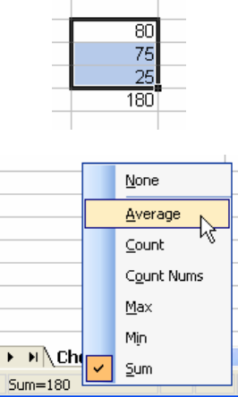
1. Drag-select cells B7:B9 and view the result in
the AutoCalculate area (right side of the
Status Bar at the bottom of the screen). The
area currently shows “Sum=180”.
2. Right-click the AutoCalculate area and
choose “Average”.
The area shows, “Average=60”.
3. Right-click the area again and choose “Min”.
The area shows, “Min=25”.
4. Right-click the area again and choose “Max”.
The area shows, “Max=80”.
5. Drag-select cells A7:B9.
6. Right-click the AutoCalculate area and choose “Count”.
The area shows “Count=6” (because six cells are selected, and all
have some data in them).
7. Right-click the area again and choose “Count Nums”.
The area shows “Count Nums=3” (because only three cells selected
have numbers in them).
Excel 2003, Level 1 Page 13
September 2005
U
U
s
s
i
i
n
n
g
g
I
I
n
n
s
s
e
e
r
r
t
t
F
F
u
u
n
n
c
c
t
t
i
i
o
o
n
n
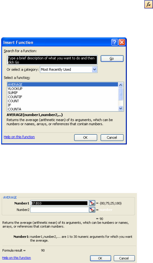
The Insert Function feature is used to get step-by-step help with choosing
a function and creating a formula.
1. Click on cell B11, and then click the Insert Function button on the
Standard Toolbar.
The Paste Function dialog box displays.
2. Note the Function Categories in the ‘select a category:’ pull down
menu. Below are displayed the functions associated with the selected
category. The “Most Recently Used” category always displays first.
3. Select “Average” from the ‘select a function:’ list and click OK.

Excel 2003, Level 1 Page 14
September 2005
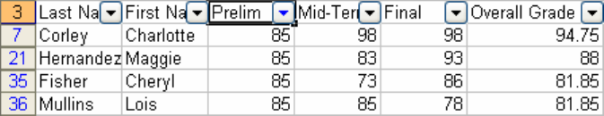
The Average Function Arguments Palette displays, showing the range
B7:B10 in its proposed formula. Because we do not want to include cell
B10 in the average, we must re-select the range of cells to be averaged.
4. Click the Collapse button
on the Function Palette.
The palette collapses to allow for better viewing of the cells on the
sheet. If necessary, move the palette bar so you can view all
desired cells.
5. Drag-select cells B7:B9 (the “line of marching ants” should go
around those cells).
6. Click the Expand button
.
The Function Palette displays again in full. The correct range of cells
is now shown in the formula.
7. Click OK to accept the formula.
The Formula Palette collapses into the Edit Line, and the results of
the formula (60) are shown in cell B11.
8. Save the file.
Section 5: Database Functions - Sorting and Filtering Data
C
C
o
o
p
p
y
y
i
i
n
n
g
g
D
D
a
a
t
t
a
a
w
w
i
i
t
t
h
h
A
A
u
u
t
t
o
o
F
F
i
i
l
l
l
l
AutoFill is a feature in Excel that allows cell contents to be copied and
updated quickly without using the copy and paste buttons.
1. Click on the “Grades” sheet tab, and select cell F4. With the cell
selected, place the mouse pointer at the bottom right corner of the cell
until the thin plus sign, called the AutoFill pointer (
) displays.
2. Click-and-drag the pointer down from cell F4 to F50.
The formula in cell F4 is copied and automatically updated to reflect
the changes needed to the formula in each new cell.
3. Save the file.

Excel 2003, Level 1 Page 15
September 2005
S
S
o
o
r
r
t
t
i
i
n
n
g
g
L
L
i
i
s
s
t
t
s
s
1. Select cell A3 (last name). Note that the records are currently in
alphabetical order.
2. Click on cell C3 (prelim grade), then click the Sort Ascending button
on the Standard Toolbar.
The records are sorted in numerical order by preliminary test score.
3. Click the Sort Descending button .
The records are sorted in reverse order.
4. Click on cell F3 (overall grade), and sort in descending order.
The records are sorted by highest to lowest Overall Grade.
NOTE:
Sort assumes that if the top cell in the column is text, that it is simply a label
that should not be sorted. If there is no text label, it sorts all data.
IMPORTANT WARNING:
DO NOT perform a sort on any table that has BLANK ROWS OR COLUMNS
(with no headings) The empty rows/columns break-up the table into “sub-
tables,” and sorting only shifts cells in one sub-table, making that chunk of
information out-of whack with the rest of the table!
Page 16
F
F
i
i
l
l
t
t
e
e
r
r
i
i
n
n
g
g
D
D
a
a
t
t
a
a
w
w
i
i
t
t
h
h
A
A
u
u
t
t
o
o
F
F
i
i
l
l
t
t
e
e
r
r
“Filtering” is the process of removing those records you do not want to see
and displaying only those records that match certain criteria. To allow
quick filtering, Excel uses a feature called “AutoFilter” for the field.
1. Select cell A3 (last name).
2. Choose Data > Filter > AutoFilter.
Excel adds AutoFilter buttons (down arrows) on each field heading.
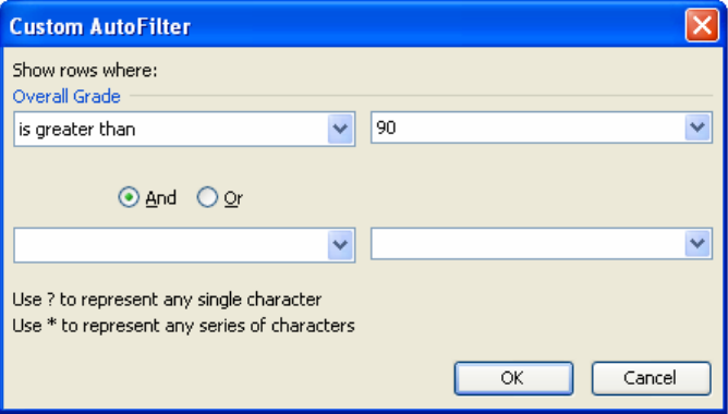
3. Click the AutoFilter button for the “Prelim” field.
A drop-down list of entries displays.
4. Select “85” from the list.
A list of students who made 85 on the preliminary exam
displays (4 students).
Note that the Plain AutoFilter button has turned blue, indicating
that it is currently in effect; also, the row headings have turned
blue, indicating that these rows match filter criteria. Rows that do
not match have been skipped.
T
T
o
o
g
g
e
e
t
t
a
a
l
l
l
l
o
o
f
f
y
y
o
o
u
u
r
r
A
A
u
u
t
t
o
o
f
f
i
i
l
l
t
t
e
e
r
r
e
e
d
d
r
r
e
e
c
c
o
o
r
r
d
d
s
s
t
t
o
o
s
s
h
h
o
o
w
w
a
a
g
g
a
a
i
i
n
n
:
:
1. Scroll to the top of the list.
2. Click the Prelim AutoFilter button, and select “(All)” from the list.
The list returns to showing all customers, and the blue filter
indicators turn off.
Excel 2003, Level 1 Page 17
September 2005
A
A
p
p
p
p
l
l
y
y
i
i
n
n
g
g
a
a
C
C
u
u
s
s
t
t
o
o
m
m
A
A
u
u
t
t
o
o
F
F
i
i
l
l
t
t
e
e
r
r
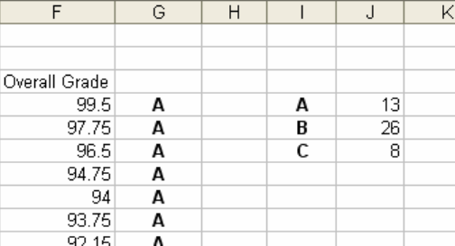
1. Click the Overall Grade AutoFilter button in cell F3.
2. Select “(Custom…)” from the list.
The Custom AutoFilter dialog box displays.
3. Click the down arrow in the “Overall Grade” area (currently reads,
“equals”).
A drop-down list of comparison operators displays.
4. Select “is greater than” from the list.
5. Click in the blank field to the right of “is greater than”.
6. Type “90”.
Enters 90 as the minimum criterion to be filtered.
7. Click OK.
The dialog box closes and applies the custom filter (13 records).
Note that it is easier to use the AutoCalculate area to determine the
total records than to manually count them on your screen!
8. Click on cell F3, then click the Sort Ascending (A-Z) button.
The records are sorted by the lowest “A” score to the highest, with
only grades better than “90” showing.
Excel 2003, Level 1 Page 18
T
T
u
u
r
r
n
n
i
i
n
n
g
g
O
O
f
f
f
f
A
A
u
u
t
t
o
o
F
F
i
i
l
l
t
t
e
e
r
r
1. Choose Data > Filter, and click the AutoFilter option, which is
currently checked.
The AutoFilter is deselected from the list.
2. Click on cell A3, then sort in ascending order.
Sorts in alphabetical order.
3. Save the workbook.
A
A
d
d
d
d
i
i
n
n
g
g
D
D
a
a
t
t
a
a
1. Sort the data in descending order of overall grade.
2. In column G, assign a grade of “A” to the first person on the list.
Bold and Center the letter A. Use Autofill to assign this formatted letter
grade to anyone else with a score of 90 or above.
3. Repeat for “B” and “C” students.
4. Create separate cells in I4:I6 for “A”, “B”, and “C”.
Enter the totals for each group in J4:J6.
September 2005

Excel 2003
Introduction
LaTonya Motley
Trainer/Instructional Technology Specialist
Staff Development
660-6452
