XLReporter Data Management

Data Management - 1 -

Data Management

Overview

Data Management provides a suite of functions that are applied to report data. They provide

numerous features such as handling of dynamic ranges, performing data analysis, and

importing/exporting from a workbook.

Usually, the Manage connections are applied after the Data connections. This ordering can be refined

by using the Group setting.

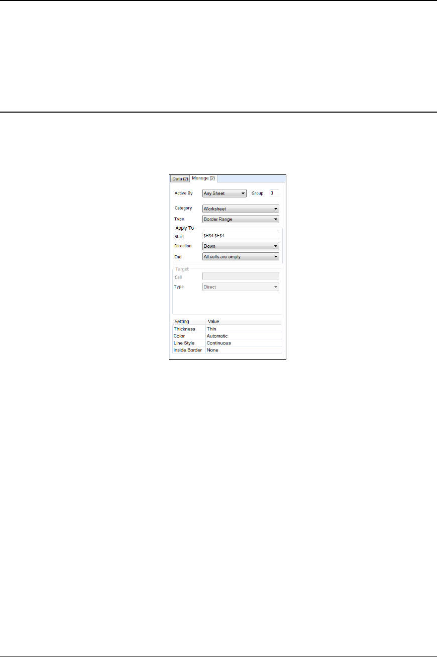
Configuration

To configure Data Management in a template, open the Design Studio and select Data, Connect. In

the Connections dialog select the Manage tab.

The Active By settings determine which worksheet or Group activates the function. With the

defaults, Any Sheet and a Group set to 0, the update of any worksheet causes the management function

to execute.

However, by setting Active By to a specific sheet, the function only activates on the update of that

specific sheet. Likewise, by setting a Group number greater than zero, the function only activates

when an action with that Group number is executed.

The available management functions are organized by Category. Each Category supports a set of

functions listed in Type.

Apply To/Source/Range

Most management functions operate on a range of data that is determined by the Apply To (Source or

Range) settings where the Start cell(s), Direction and the End condition collectively determine the

range at runtime.

• Start

This defines the initial range. It can be a single cell, single row, single column or a range of

multiple rows and columns. This range is then expanded based on the Direction and End

Conditions.

Data Management - 2 -

• Direction

This determines the direction in which the Start range is expanded. The following options

may be available depending on the management function selected.

• None

No expansion is done. The Start range is used as is.

• Down

The Start range is expanded down based on the End criteria.

• Across

The Start range is expanded across based on the End criteria.

• Down (variable columns)

The Start range is first expanded across the columns based on the End criteria, then

expanded down using the same End criteria.

• Across (variable rows)

The Start range is first expanded down the rows based on the End criteria, then

expanded across using the same End criteria.

• End

This determines when the expansion of the range stops. Note that if multiple rows or columns

are specified in the Start range, the End criteria is applied starting at the bottom row or

rightmost column depending on the Direction.

• Edge cell is empty

The range is expanded until the first empty cell in the leftmost column or topmost

row (depending on Direction) is found.

• All cells are empty

The range is expanded until the first entirely empty row or column (depending on

Direction) is found.

• First empty cell

The first empty cell in each row (or column) is determined and then the range is

expanded to the topmost (or leftmost) cell relative to the range.

• Last empty cell

The last empty cell in each row (or column) is determined and then the range is

expanded to the bottommost (or rightmost) cell relative to the range.

For example: A history data group connection placed in $B$4 provides a date/time and 4 columns. If

a border is required around the report data then the Apply To settings are $B$4:$F$4, Down, All cells

are empty.

Placement

Management functions that produce output, such as Copy Range, require a Placement to determine

where the output is placed.

The Cell location determines the placement. The Type indicates how the placement is performed.

The following Types are available:

• Direct

The output of the function is placed directly into the cell given by the Cell.

• Offset

The output of the function is placed in a row or column (see Direction) relative to the Cell

according to the value of the Offset. The Offset can be an XLReporter counter variable

(e.g., CR000) or a time-based calculation (e.g., mM/15, 15 minute offset of the month).

• Append

The output of the function is appended onto the end of the existing data in the row or column

relative to the Cell according to the Direction.

• Insert At Start

The output of the function is inserted at the Cell in the specified Direction. Any content

below or to the right of the insertion is moved down or across.

Data Management - 3 -

• Insert At End

The output of the function is inserted at the end of the existing data in the row or column

relative to the Cell according to the Direction. Any content below or to the right of the

insertion is moved down or across.

• Insert At Start (full)

The output of the function is inserted at the Cell in the specified Direction by inserting entire

rows or columns (depending on Direction). Any content below the Cell row or to the right of

the Cell column of the insertion is moved down or across.

• Insert At End (full)

The output of the function is inserted at the end of the existing data by inserting entire rows or

columns in the row or column relative to the Cell according to the Direction. Any content in

rows below the Cell row or to the right of the Cell column is moved down or across.

Cell References

In the above, the Cell determined the placement. This can be expressed in two ways.

• Absolute Cell Reference

The setting can be either fixed text or a cell reference, the cell reference must be an absolute

reference (e.g., $A$1).

• Named Cells/Ranges

For any cell reference setting, a Named Cell/Range can be used. The advantage of using a

named cell or range is that if rows or columns are inserted or deleted from the worksheet, the

named cell or range is shifted accordingly.

For more information on how to configure named cells and ranges, see the Named

Cell/Range section of the Template Studio document under the DESIGN category in the

Document Library.

Variables and Name Types

Any function setting that supports a hard coded value can also be set with a Variable or Name Type.

Order of Operations

By default, management connections are updated after the data connections so that the management

connections can operate on the data brought in by the data connections.

To change order in which connections are updated, use the Group setting for both the data and

management connections and then configure the Update Group actions accordingly.

Data Management - 4 -

Data Management Reference

Worksheet

This set of Data Management functions are when dynamic ranges are used i.e., when the number of

data rows/columns cannot be predicted. Dynamic ranges are commonly found in discrete reports,

reports over a batch, or on-demand reports where the user specifies the report parameters.

The handling of dynamic ranges can be achieved by using an Insert Placement of a data connection,

but these functions provide more custom functionality.

AutoFit Range

The AutoFit Range function adjusts either the column widths or row heights of the range determined

by the Apply To settings based on the content of the cells in the range. This can be very useful if the

report contains a data group which brings in either headers or textual data that can vary in size.

Settings

AutoFit

• Column Width

Each column in the range is widened based on the cell in the column with the largest

amount of data (e.g., the cell with the most characters).

• Row Height

Each row in the range is adjusted in height based on the cell in the row with the largest

amount of data (e.g., the cell with the most characters).

This setting is most effective if the cells are formatted to wrap text.

Example

A report template is designed to allow the user to select tags which are displayed in the report. Since

tag names will vary in length it is difficult to size the column widths ahead of time. Instead, an

AutoFit Range management function is configured to run after the data is retrieved.

If the report data is configured for cell $B$8 with an additional 12 columns, the AutoFit Range

function is configured as:

Apply To $B$8:$N$8, Down, All cells are empty

Setting

AutoFit Column Width

Border Range

The Border Range function draws a border around the outside (and optionally inside) of the Apply To

range.

Settings

Thickness

The thickness of the border to draw.

Color

The color of the border to draw. This can either be Automatic (based on the theme of the

template), a specific color listed or a numeric color in the R,G,B format. For example, the RGB of

a gray border is 128,128,128.

Data Management - 5 -

Line Style

The style of the border lines drawn which can be Continuous for single lines or Double for double

lines.

Inside Border

This determines if inside borders are applied to the range. These can be applied just the Columns

of the range, Rows of the range or Both rows and columns in the range.

Example

A batch report template is created to retrieve 1 minute samples over the duration of the batch from

historical data. A border should be drawn around the data for completeness. Since batches run at

different durations, the border cannot be drawn on the template. This function is used to draw this

border after the data is retrieved. Data starts on $B$8:$H$8. The settings for the function are:

Apply To $B$8:$H$8, Down, All cells are empty

Setting

Thickness Thin

Color Automatic

Line Style Continuous

Inside Border None

Chart Range

The Chart Range function adjusts chart settings, such as data series ranges, of an existing chart in the

workbook using the Source.

If the data series ranges do not need to be adjusted but the chart needs its X or Y axis to be adjusted,

use the Chart Enhancement function under the Placement category.

Settings

Chart Name

The name of the chart to apply the function to. The browse button (…) opens a list of every

configured chart within the workbook to select from. The list is in the format:

Chart Name – Sheet!Range of the chart

If a chart is selected in the list, the worksheet for the chart is activated and the range of the chart is

selected to highlight the chart itself.

The chart name is not visible and is typically not set by the user. When a chart is inserted into a

worksheet it is given a default name (Chart X where X is a number that starts at 1). However, if

the worksheet is copied to another sheet, if the default name is left it can be changed on the new

worksheet. To combat this, charts in the template are renamed to a fixed name (xlrX where X is a

number that starts at 1) so that chart names are consistent between worksheets.

Note that only charts configured to worksheets are listed. Charts configured on a Chart Sheet

cannot be used with this function.

Add/Remove Series

If set to Yes, when the function is executed, it will ensure that the number of series in the chart

match the number of columns (or rows depending on Direction) in the Source range.

If there are more series configured than there are columns (or rows) in the Source range, the extra

series are removed.

If there are less series configures than there are columns (or rows) in the Source range, those

series are added to chart. The series properties like color, weight, thickness, etc. are determined

by the defaults of the Design Studio.

Data Management - 6 -

The rule of thumb here is that if you want total control over the formatting of every series set up

the chart for the worst case and let this function remove unused series. Otherwise just set up the

first series and let this function add the others as needed.

X-Axis Ticks

The number of tick marks and labels displayed on the X-axis of the chart. Set this to 0 to

automatically determine the number of tick marks and labels.

Adjust Y-Axis

The scaling of the Y-axis of the chart. Set to None to use the default scaling set for the chart,

Automatic to determine the minimum and maximum as the minimum/maximum of the values of

the series plus +/- 1% or Custom to use cell values for the minimum and maximum.

Y-Axis Minimum

If Adjust Y-Axis is set to Custom this setting must be set to a cell reference containing the

minimum scale value for the Y-Axis.

If the chart has a secondary axis, the minimum scale value for it can be specified as a range of two

cells either horizontally or vertically. E.g., $B$4:$B$5 means that the minimum for the primary

axis comes from cell $B$4 and the minimum for the secondary axis comes from cell $B$5.

Conversely a range of $B$4:$C$4 means that the minimum for the primary axis comes from cell

$B$4 and for the secondary comes from cell $C$4.

If the cell is not on the Active By sheet, the sheet must be specified, e.g., Sheet1!$B$5.

Y-Axis Maximum

If Adjust Y-Axis is set to Custom this setting must be set to a cell reference containing the

maximum scale value for the Y-Axis.

If the chart has a secondary axis, the maximum scale value for it can be specified as a range of two

cells either horizontally or vertically. E.g., $C$4:$C$5 means that the maximum for the primary

axis comes from cell $C$4 and the maximum for the secondary axis comes from cell $C$5.

Conversely a range of $C$4:$D$4 means that the maximum for the primary axis comes from cell

$C$4 and for the secondary comes from cell $D$4.

If the cell is not on the Active By sheet, the sheet must be specified, e.g., Sheet1!$B$5.

Example

An On-Demand report template is created where the user can select the time period and up to 8 tags to

display both the data and as series on a line chart. Because of the variability of both the length of each

series as well as the number of series (e.g., if only 4 tags are selected only 4 series should be shown),

the chart cannot be fully configured ahead of time in the template. Instead, the chart is configured for

8 series where the range for each series in set to just the top row where the data is written. A Chart

Range function is used to both adjust the range of each series as well as remove series that are not

used. If the data starts in $B$8:$J$8, the settings for this function are:

Source $B$8, Down (variable columns), All cells are empty

Setting

Chart Name xlr1

Add/Remove Series Yes

X-Axis Ticks 0

Adjust Y-Axis No

Clear Range

The Clear Range function clears various elements of the Apply To range.

Data Management - 7 -

Settings

Clear

• All

Everything the range is cleared including content and any applied formatting.

• Contents

The content of every cell in the range is cleared. This is the equivalent of highlighting a

range of cells and pressing the Delete key.

• Formats

All formatting including font size, style, color as well as background color and any

conditional formatting is cleared from the cell. The content in the cells remains.

• Errors

This option clears cells containing the error #REF or #DIV/0! In the case of #DIV/0 the

cell content is cleared. In the case of #REF the part of the formula that is causing the

#REF is removed to correct it. For example, if cell contains the equation

=$A$3+$A$4+#REF then it will become =$A$3+$A$4. If the formula cannot be

corrected, then it is cleared.

Example

A live dashboard template is configured which always shows the last 10 temperature readings from a

tank with the most recent value on top and the previous 9 below. The data connection that brings in

the temperature is set up to Insert At Start with a Direction of Down. Since 10 values need to be

shown the report cannot be overwritten every time but once 10 rows are filled, for every update the

value should “drop off” leaving the last 10. This can be accomplished using a Clear Range

function. If the value starts in cell $B$4 the 10

value is in $B$13. The settings for the function are:

Apply To $B$14, None

Setting

Clear All

Collapse Range

The Collapse Range function removes empty columns from the Apply To range. Before collapsing,

any cells containing #REF that cannot be corrected are also cleared.

Settings

Extend Rows

This extends the rows of the Apply To range before determining if the column is empty and

therefore removed. The syntax is: Rows Above, Rows Below, e.g., 2, 1 to extend the Apply To

range 2 rows above and 1 row below what is initially determined.

Adjust Column Widths

If set to Yes, after collapsing the remaining columns widths are adjusted to fit the data in the

column.

Border Range

This setting allows for an outside border to be drawn around the range after it is collapsed.

The border is a thin, continuous (single line) border using the Automatic color.

Data Management - 8 -

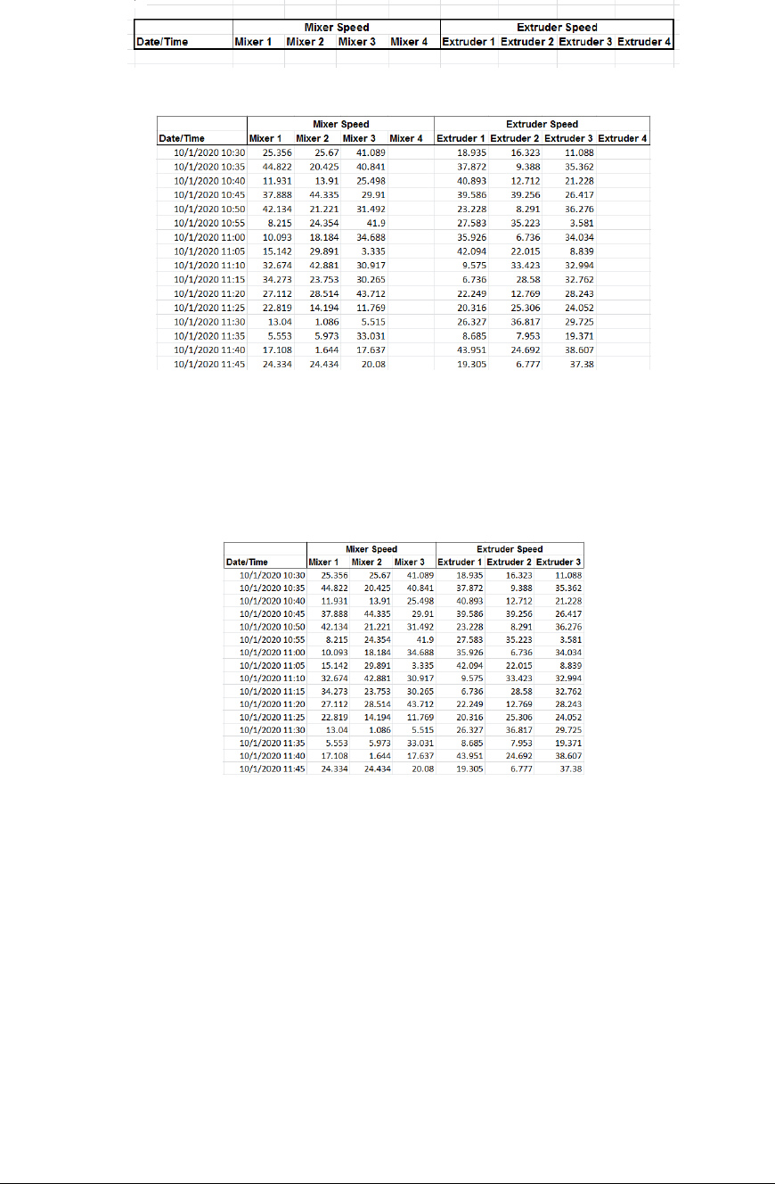
Example

A plant has 3 production lines. Line 1 has 3 mixers and 3 extruders. Line 2 has 4 mixers and 2

extruders. Line 3 has 2 mixers and 4 extruders.

Instead of creating a template for each line, create a single template for the worst-case scenario (4

mixers and 4 extruders).

When the report is generated for Line 1 the header is placed in row 1, data is placed in row 3 and

empty columns for Mixer 4 and Extruder 4 (since this line does not have these assets):

Now apply the collapse range with these settings:

Apply To $B$3:$J$3, Down, All cells are empty

Setting

Extend Rows 1,0

Adjust Column Widths No

Border Range No

Condense Range

The Condense Range function condenses a table of data based on a column and a Group Method.

Settings

Group

The cell that defines the column within the Apply To range used to condense the data in the other

columns.

Group Method

The method by which to group the data in the Group column. The Group column can contain

text, numbers, or timestamps. Text can be grouped with or without case sensitivity.

Data Management - 9 -

For numbers, grouping can be done on the Cell Value or the Cell Text (case is not considered

here).

• Cell Value

Grouping is based on the underlying value in the cell, to the accuracy of the cell value

• Cell Text

Grouping is based on the cell value displayed (and formatted).

For example, if the Group column has the values 2.11 and 2.12 and formatted for 1 decimal

place, Cell Value would treat these as different whereas the Cell Text would treat them the

same.

For timestamps, the Group Method can be Second, Minute, Hour, Day, Month or Year in

multiples of the Interval.

Condense To

This defines how to condense the data in the columns in the range outside the Group column.

The following options are available:

• First Value

The value corresponding to the first row of the group.

• Last Value

The value corresponding to the last row of the group.

• Average

The average of all the rows of the group.

• Maximum

The maximum value of all the rows in the group.

• Minimum

The minimum value of all the rows in the group.

• Total

The total of all the rows of the group.

• Count

The count of all the non-blank rows of the group.

Interval

This setting can be a fixed number, a variable, or a single cell reference. If Interval does not

evaluate to a number, it is set to 0.

The value of Group Method and Interval influence how the grouping is performed.

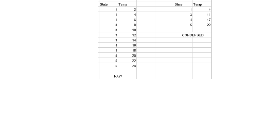
• Cell Value

o Interval = 0

Rows are condensed for each unique value in the Group column.

In the above example, the Temperature is averaged over each unique State.

Data Management - 10 -

o Interval > 0

The rows are condensed in groups that are determined by the value of the first row of

the Group column plus a multiple of the interval.

In the above example the Interval=1 which results in the Temperature averaged over

every State., leaving blanks in the result e.g., State=2 does not exist in the raw data.

• Cell Text

o Interval (not used)

Rows are condensed for each unique displayed value in the Group column.

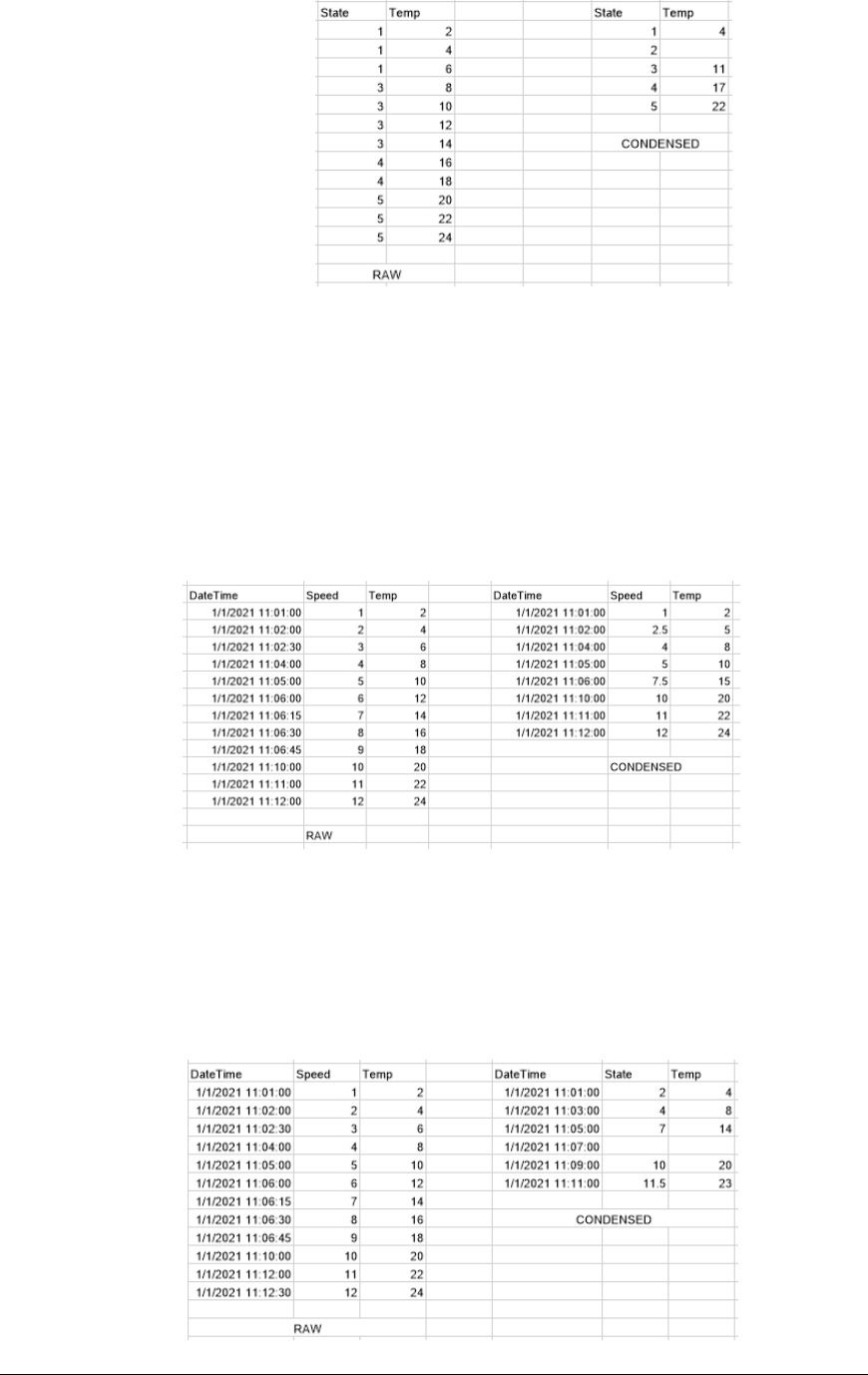
• Time Based

o Interval = 0

Rows are condensed for each unique value of the selected time element in the Group

column. For example, suppose a Group Method of Minute and an Interval of 0.

In the above example, the raw data is condensed to averages for each unique minute

in the DateTime column.

o Interval > 0

The rows are condensed in groups that are determined by the value of the first row of

the Group column plus a multiple of the Interval of the Group Method selection

In the following the Group Method is Minute and the Interval=2.

Data Management - 11 -

In the above example, the raw data is condensed to averages for each 2 Minute

interval in the DateTime column. In the absence of data in the group, an empty

record is displayed e.g., 11:07:00.

Example

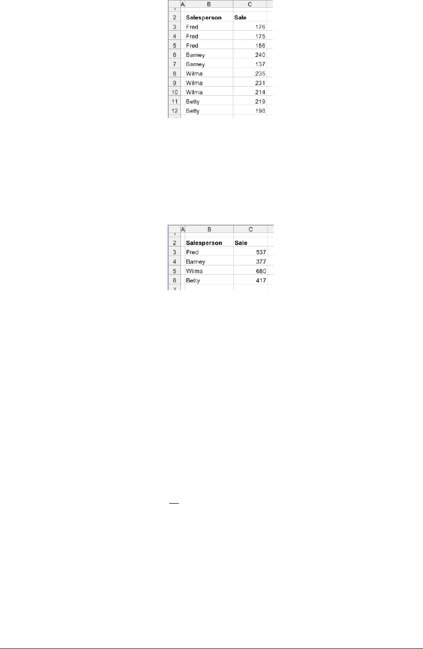
Consider the following table of data:

To calculate the total sales for each person, use the following settings:

Apply To $B$3:$C$3, Down, All cells are empty

Setting

Group $B$3

Group Method Cell Text (Case Insensitive)

Condense To Total

Interval 0

Copy Range

The Copy Range function copies the Source range and pastes it to the Placement using the Type

operation such as Direct, Offset, Append, and Insert.

If the Placement Type is Insert At Start (full) or Insert At End (full) the entire rows or columns

(depending on Direction) are copied from the Source and pasted.

The Placement can be either:

• Cell

Select this option if the placement is to a fixed cell e.g., $B$17

• Name

Select this option if the placement is to a named cell. To name a cell, right click on the desired

cell and select Define Name.

Any row/column insertion that happens above or to the left of a named cell will cause name

cell location to change accordingly. Special consideration is given to a cell named LastCell

since a row/column insertion on this name cell causes the location to change by the number of

rows/columns inserted.

Settings

Paste

The Paste option determines what is copied to the Placement from the Source.

• All

Everything from the range including the cell contents (values and formulas), formatting,

charts and validation is copied and pasted to the Placement cell.

• All Except Borders

Everything from the range except for borders is copied and pasted to the Placement cell.

Any existing borders in the Placement range will remain.

Data Management - 12 -

Note, charts within the Source range are not copied and pasted with this setting. The All

setting must be used to copy charts.

• Formulas

The content from the range is copied and pasted to the Placement cell. Any formulas in

the range are pasted. Any existing formatting in the Placement range will remain.

• Formulas and Formats

The content and formatting from the range is copied and pasted to the Placement cell.

Any formulas in the range are pasted.

Data Management - 13 -

Validation

The data validation from the range is copied and pasted to the Placement cell. Any

existing formatting in the Placement range will remain.

• Validation and Formats

The data validation and formatting from the range is copied and pasted to the Placement

cell.

• Values

The content from the range is copied and pasted to the Placement cell. Any formulas in

the range are replaced with the result of the formula. Any existing formatting in the

Placement range will remain.

• Values and Formats

The content and formatting from the range is copied and pasted to the Placement cell.

Any formulas in the range are replaced with the result of the formula.

• Formats

The formatting from the range is copied and pasted to the Placement cell.

Operation

If the copy is performed to a Placement that already contains values, the Operation determines

how the copy will occur. Set the Operation to None to copy the Source over the Placement

whereas the selection of an arithmetic Operation combines the values from the Source and

Placement ranges.

Transpose

Setting Transpose to Yes transposes the Source before it copied to the Placement. In this case

the Source and Placement cannot overlap or this function generates an error. Note, when

Placement is set to Yes, no charts are pasted if the Paste option is set to All.

Skip Blanks

Setting Skip Blanks to Yes prevents empty cells in the Source overwriting cells in the Placement.

For example: Copying cells D5:F5 with E5 empty to the range A1 to C1 does not overwrite the

value in cell B1 (since E5 is empty).

Clear Data

The Clear Data setting can be set to clear the Source range after it is pasted. The following

options are available:

• No

Nothing is cleared from the Source range.

• All

Everything is cleared from the Source range. This includes any values, formulas, and

formats.

• Contents

The content of every cell in the Source range is cleared. This is equivalent of

highlighting a range of cells and pressing the Delete key.

Adjust Column Widths

If set to Yes, the column widths of the Placement range are adjusted to match the Source range.

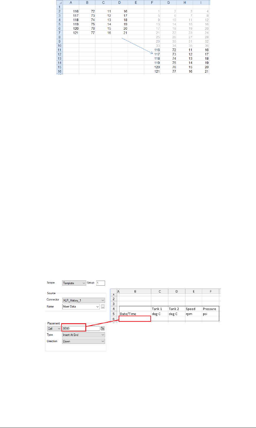
Example

To copy a number of rows of data starting at $A$2:$D$2, paste them to the next empty cell at or

beneath $F$4.

Data Management - 14 -

Use the settings:

Source $A$2:$D$2, Down, All cells are empty

Placement $F$2, Append, Down

Setting

Paste All

Operation None

Transpose No

Skip Blanks No

Clear Data No

Adjust Column Widths No

Copy Sub Report Range

The Copy Sub Report Range function behaves like the Copy Range function in that the content of

the Source range is copied and pasted to the Placement defined. This includes any content,

formatting, formulas, charts, column widths, row heights and outlining.

This function also copies any data connections in the Source, either Data or Manage.

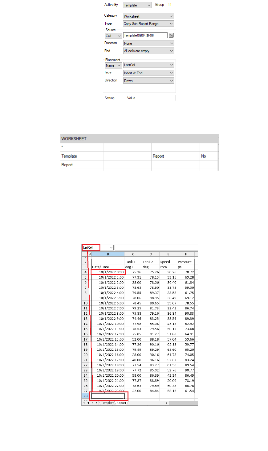
Example

A template workbook is configured with two sheets: Template and Report.

The Template has a content in a range of cells in B4:F6 with a history connection in cell $B$6

(assigned to Group 1).

The Mixer Data history group in this example is defined to return 24 rows.

A Copy Sub Report Range management connection is configured to copy the range $B$4:$F$6 from

the Template sheet to the named cell LastCell on the Report worksheet (assigned to Group 11). .

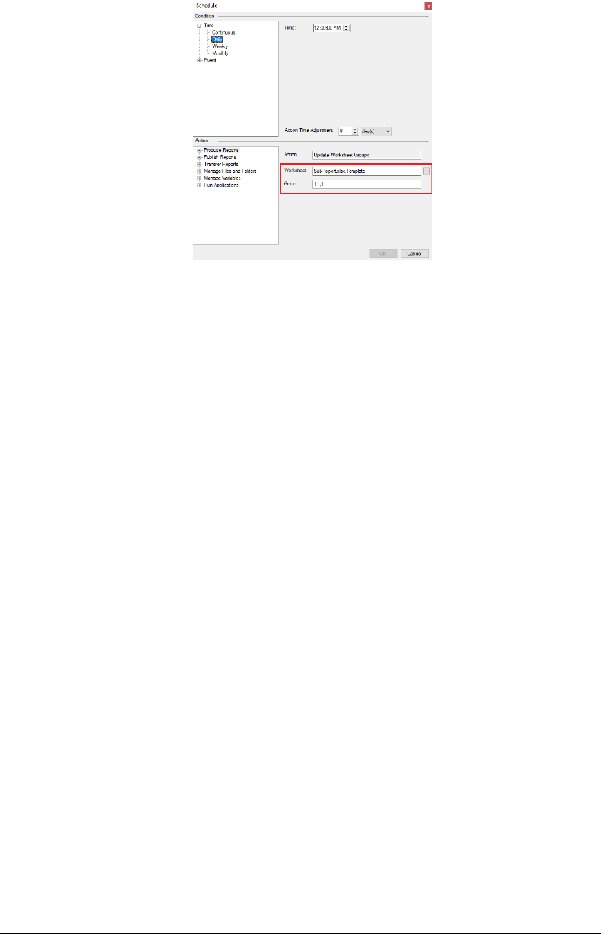
Data Management - 15 -

The Report Names are defined with the target worksheet of Template is Report so any data connection

applied to the Template sheet is copied to Report.

When the Copy Sub Report Range function is performed, $B$4:$F$6 from Template is copied to

LastCell $B$2 in Report (see the Placement Name above).

When the template is processed by an update of Group 11 followed by a Group 1 the following

happens:

• The sub report is copied from the Template to the call Last Cell in the Report (group 11)

• The history data is added to the Report (group 1)

• Because the history data is configured to Insert, the cell Last Cell is moved down in Report

equal to the number of rows inserted.

If this process is repeated to different sub reports (each with its own connections) and they target

LastCell, a stacked report of varying sub reports can be achieved.

Data Management - 16 -

To initiate the processing from the scheduler, the Update Worksheet Groups Action is used with the

appropriate group numbers e.g., 11,1.

From the scheduler this would be:

Cut Range

The Cut Range function cuts the Source range and pastes it to the Placement Cell using the Type

operation such as Direct, Offset, Append, and Insert. All formats, formulas and values from the

Source are pasted to the Placement.

Note, charts within the Source range are not cut and pasted with this function.

Settings

Delete Range

If set to Yes then the Source range is deleted after it is cut and pasted rather than just cleared from

the worksheet.

Shift Cells

If Delete Range is set to Yes, this determines how the cells are shifted after the range is deleted,

either Up or Left. Otherwise, this setting has no effect.

Example

To cut a number of rows of data starting at $A$2:$D$2, paste them to the next empty cell at or beneath

$F$4.

Source $A$2:$D$2, Down, All cells are empty

Placement $F$2, Append, Down

Setting

Delete Range No

Shift Cells Up

Delete Range

The Delete Range function deletes the Apply To range from the worksheet. The difference between

delete and clear is that delete physically removes the cells from the worksheet rather than just clearing

them of content and formatting. When a range is deleted it affects any formulas or charts that may be

configured for the range.

Settings

Shift Cells

This determines how the cells are shifted after the range is deleted, either Up or Left.

Data Management - 17 -

Example

A live dashboard template is configured which always shows the last 10 temperature readings from a

tank with the most recent value on top and the previous 9 below along with a chart graphically

displaying these values. The data connection that brings in the temperature is set up to Insert At Start

with a Direction of Down. Since 10 values need to be shown the report cannot be overwritten every

time but once 10 rows are filled, for every update the 11

value should “drop off” leaving the last 10.

In this case a Delete Range function must be used rather than a Clear Range so that the range of the

chart series does not expand as data is brought into the report. If the value starts in cell $B$4 the 10

value is in $B$13. The chart series values are set to $B$4:$B$5. The settings for the function are:

Apply To $B$14, None

Setting

Shift Cells Up

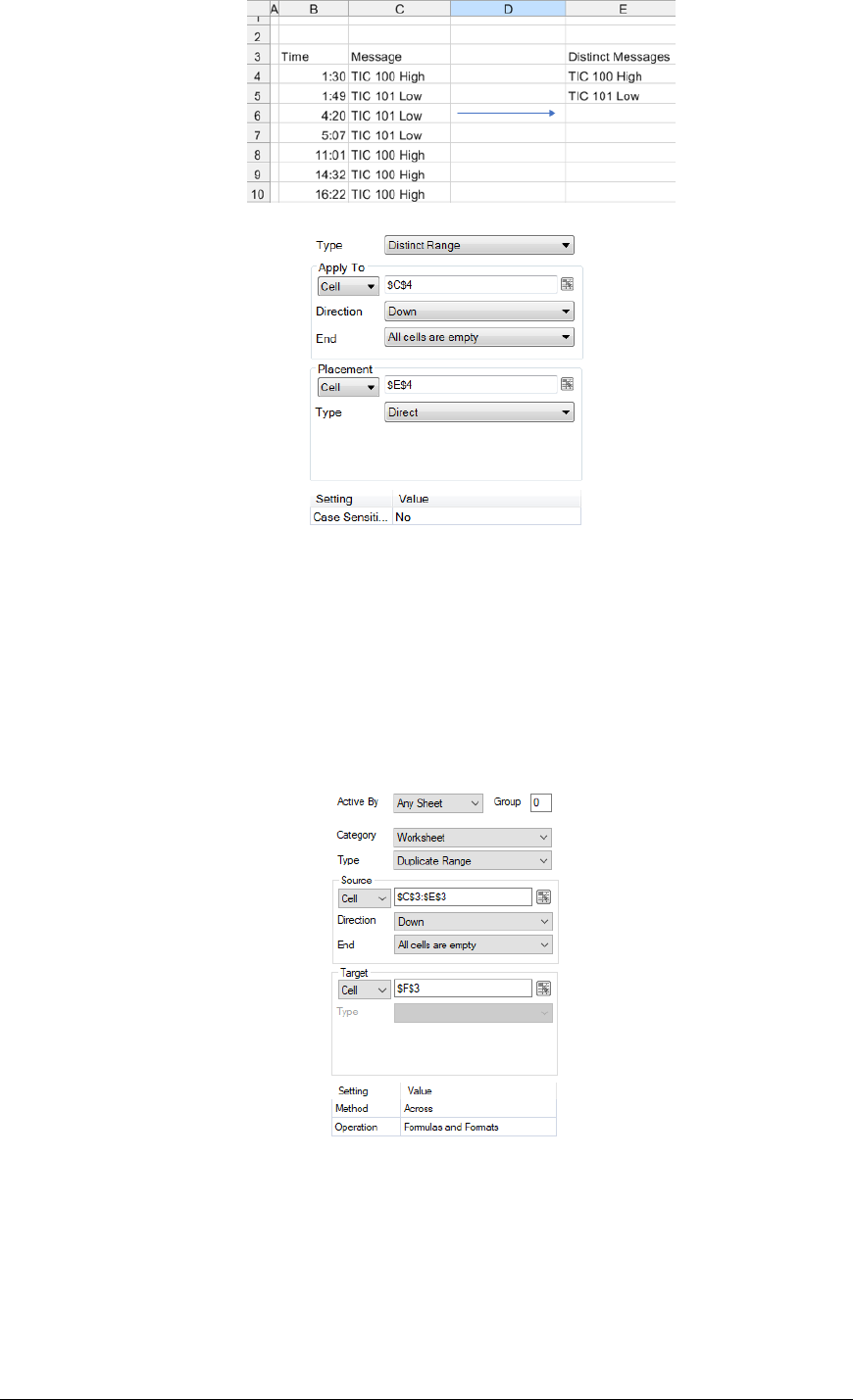
Distinct Range

This function produces a distinct list of values from a row or column of data (depending on the Apply

To Direction setting).

Note that the list is determined from the content seen in the cell which means that if the values are

numeric and formatted to a fixed number of decimal places, multiple values could be considered the

same number (even though their decimal value is different).

Settings

Case Sensitive

If the values are textual, this determines if case is considered.

Example

A daily alarm report shows every alarm that occurred over the day. A list of distinct alarms

targets focus on what needs attention.

Data Management - 18 -

Result

Settings

Duplicate Range

The Duplicate Range function performs a duplication of layout content containing the formats and/or

formulas of the Source range to the range starting at the Target cell specified.

The extent of the duplication is determined by a combination of the Source range size and the Method

specified in the Setting.

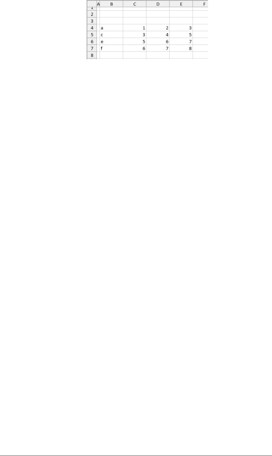
For example, suppose the Source range is three columns wide by six rows high and the Method is

Across as follows:

When this connection is processed (usually after a data connection has placed content on the report),

the Source range is determined by starting at C3:E3 and expanded Down until All cells are Empty. The

determined Source range is then copied to the Target Cell repeatedly Across the data until empty cells

in three columns and six rows is reached i.e., the size of the Source.

Settings

Method

The Method specifies the direction used to determine the Target starting at the Target Cell.

Operation

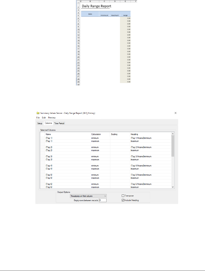
Data Management - 19 -

The Operation indicates the elements of the Source range to duplicate to the Target.

• Formats

Duplicate the cell formatting from the Source including (but not limited to) Number Formats,

Font settings, Borders, Conditional Formatting and Data Validation.

• Formulas

Duplicate any formulas from the Source to the Target using the same relative cell location.

Example

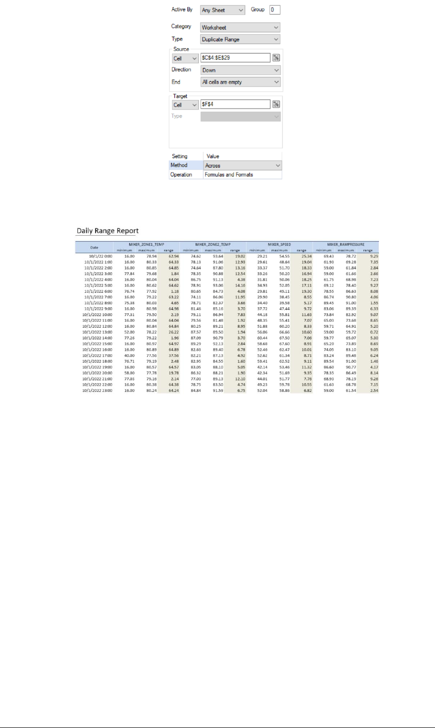
A template is configured for a user to select up to twelve tags from a historian to create a daily report.

For each tag, the hourly minimum and maximum values are shown and on the report with the

difference (delta). The template would look something like the following.

In the above, the E column contains a formula for the difference between the maximum and minimum.

A history data group is used for values, connected Directly to cell $B$4.

The Column setting of the history group is:

Note the empty row prevents the difference formula from getting overwritten.

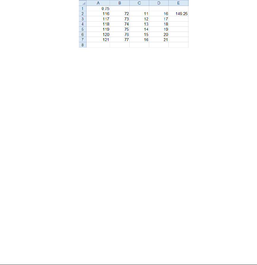
The template is set up with formatting in the range C4:E29 and a Duplicate Range function is used to

duplicate the formatting and formulas in this range across for the first tag to all the other selected tags.

Settings

Data Management - 20 -

Results

The completed report would look something like the following:

Fill Range

The Fill Range function fills cells across rows or down columns as defined by the Base range with

values as defined in the Formulas setting.

This is the equivalent of using the fill option (or fill tool) in the worksheet to drag formulas or values

down or across cells.

Settings

Formulas

The range of cells containing the formulas (and/or values) to fill. If the Formulas contain

absolute cell references, such as $B$4, they remain fixed during the fill operation otherwise they

are adjusted as the cells are filled.

Place Formula

If set to No after the cells are filled the formulas are removed from the cells so only the values

remain. Otherwise, formulas are left in the cells.

Apply Formatting

• None

No formatting is applied to the filled range.

• All

All the formatting from the Formulas range is applied to the filled range.

• All Except Borders

Data Management - 21 -

All the formatting except the borders from the Formulas range is applied to the filled

range.

Fill

This setting defines whether only cells containing Formulas are filled or if All cells are filled

regardless of content. This can be really helpful if you have formulas interspersed with your data

and want to use a single Fill Range to fill the formulas down but ignore the values themselves.

Placement

This setting determines the placement of the formulas when they are filed.

Direct means that the formulas are directly written to the cells beneath or to the right (depending

on Direction) from the original Formulas. If there is any content in these cells, it is overwritten.

Insert At End means that before the formulas are written to the cells, the range is inserted, and

cells are shifted either down or across (depending on Direction) then the formulas are filled. This

means that any other formulas or charts that depend on the values from these formulas are

automatically resized for the number of rows or columns inserted.

Example

The formula at cell E2 is =SUM(A2:C2)*$A$1 (note that $A$1 will not change during the fill).

To fill the formula to row 7, use the settings:

Base $A$2:$D$2, Down, All cells are empty

Setting

Formulas $E$2

Place Formula No

Apply Formatting All

Fill All

Placement Direct

Filter Range

The Filter Range function applies filtering to the Apply To range removing any row or column of

data (based on Direction) that does not satisfy the Condition defined.

Settings

Filter

This defines how to filter Condition is applied to the range.

• Value

The Condition is applied to the values in every row or column (depending on Direction)

in the range.

• Difference

The filter is applied to the difference in value between the row and row below or column

and column across (depending on Direction) in the range.

Condition

Data Management - 22 -

This defines the condition of the filter. Only values in rows or columns (depending on Direction)

that satisfy this condition remain, all other rows or columns are removed.

The condition is defined in the Filter Browser (see details below).

Type

This setting is only applicable when Filter is set to Difference.

• Raw

Each consecutive row (or column) of values is evaluated for the Condition.

• Deadband

As rows (or columns) are evaluated, once a consecutive set of values does not satisfy the

Condition, rows beneath (or columns to the right) are calculated against the first row (or

column) that did not satisfy the Condition.

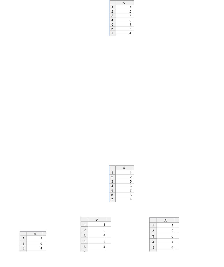
Consider the following range of values:

If the Condition is $A = 1 and the Type is Raw rows 2, 3, 5 and 6 would not meet the criteria and

be filtered out.

However, if Type is Deadband, rows 2, 3, 4 and 5 would not meet the criteria and be filtered out.

Display

This setting is only applicable when Filter is set to Difference.

• All

If the Condition is not satisfied, both the leading and trailing rows (or columns) are

removed from the range.

• Leading

If the Condition is not satisfied, the leading rows (or columns) are removed from the

range.

• Trailing

If the Condition is not satisfied, the trailing rows (or columns) are removed from the

range.

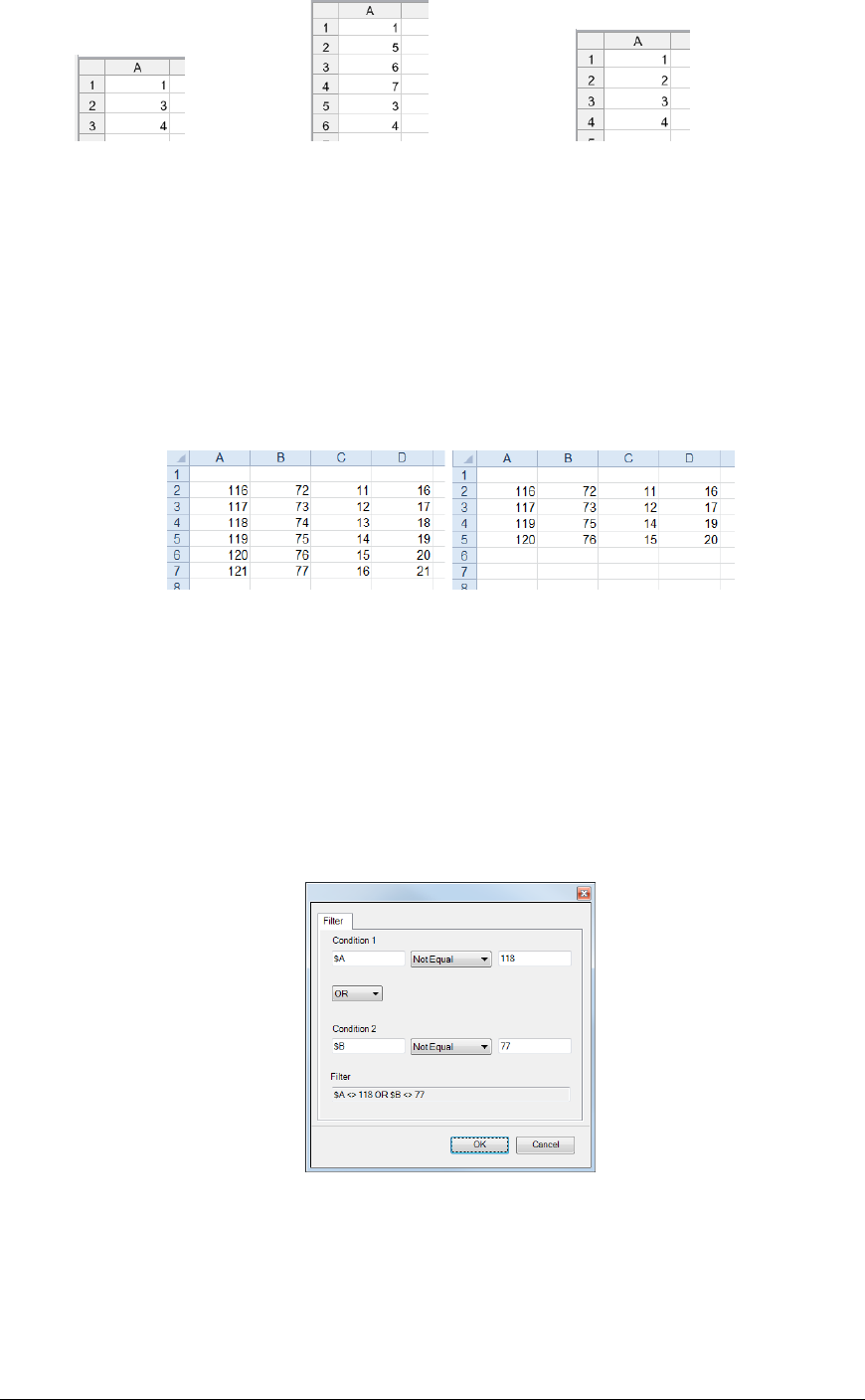
Consider the following range of values:

If the Condition is $A = 1 and the Type is Raw the results are:

All Leading Trailing

Data Management - 23 -

If the Type is Deadband, the results are:

All Leading Trailing

Case Sensitive

If the Condition is textual, this defines if case should be considered when evaluating the filter.

Delete Records

If set to Yes then every record (row or column) that does not meet the Condition is deleted

shifting every row beneath it up or every column to the right upwards or to the left (depending on

Direction). This means that any additional data beneath or to the right of the filtered range is

shifted as well. When set to No, any addition data beneath or to the right of the filtered range is left

in place.

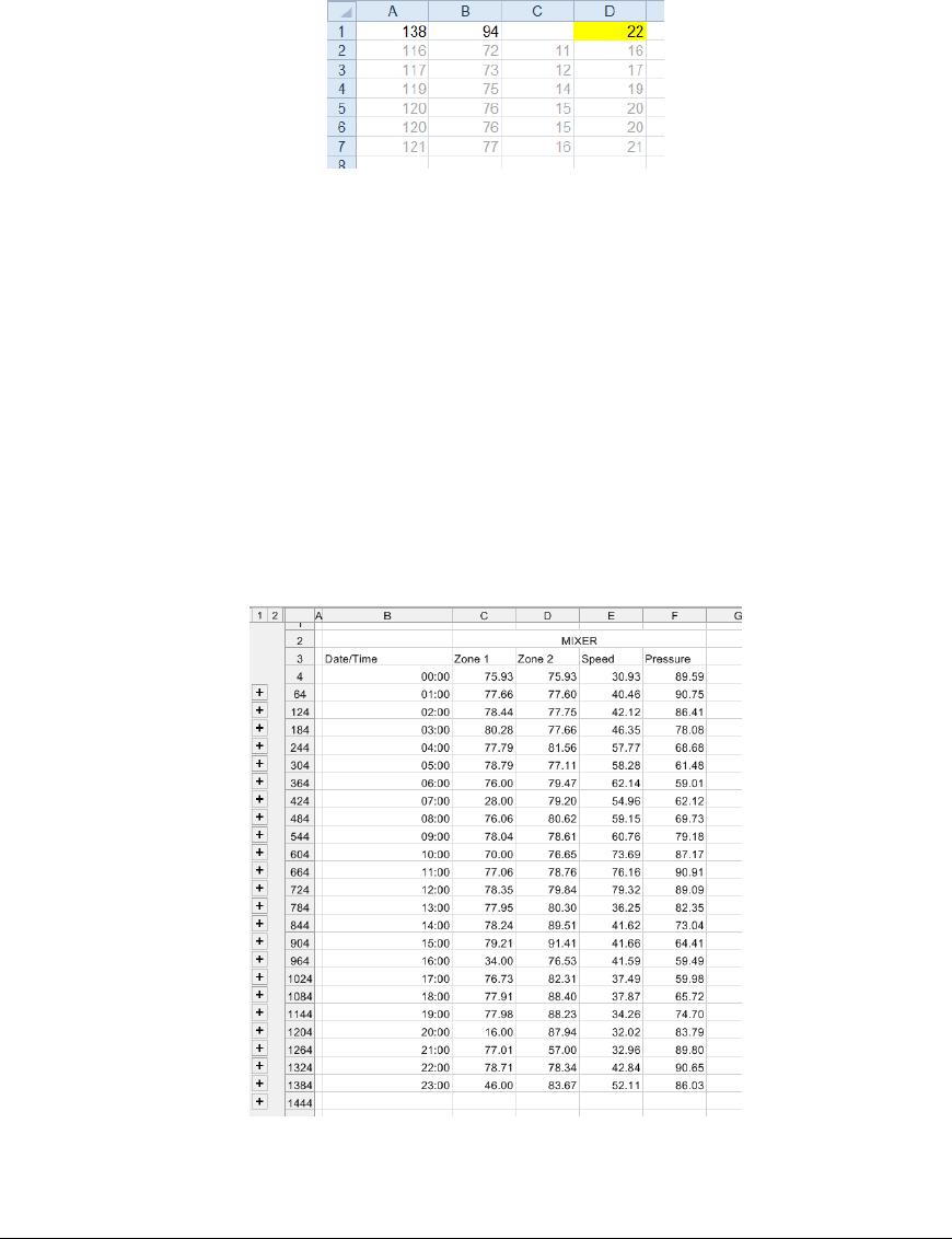
Example

Filter the filter A<>118 or B<>77 starting on row 2.

Use the settings:

Apply To $A$2:$D$2, Down, All cells are empty

Setting

Filter Value

Condition $A<>118 OR $B<>77

Type Raw

Case Sensitive No

Delete Records No

Filter Browser

The Filter Browser is used to construct filter conditions. The values can be hard coded number, text

string, cell references or XLReporter variables. When filtering text values using LIKE or NOT LIKE

operators, the wild card (%) can be used. For example, %ABC% filters any text containing ABC,

whereas %ABC filters any text ending with ABC.

Format Range

Data Management - 24 -

The Format Range function applies formatting to the Apply To range. This includes any conditional

formatting configured.

Settings

Based on

This determines range within the Apply To range to get the formatting from. This can either be

the Topmost Row or Leftmost Column of the range.

Adjust Column Widths

When set to Yes, the column widths of the Apply To range is resized based on its content. This is

only applicable when Direction is set to Across.

Stripe Color

If set, the background color added to the range at the Stripe Interval specified. This can either be

a specific color listed or a numeric color in the R,G,B format. For example, a gray stripe could be

specified as 128,128,128.

Stripe Interval

If a Stripe Color is specified this defines the interval at which to apply the striping. If the

Direction is Down this interval represents rows. If the Direction is Across this interval represents

columns.

Border Range

If set to Yes, an outside border is added to the range. The border is thin, continuous and uses the

Automatic color setting. If something more specific is required, set this to No and configure a

Border Range function.

Example

A batch report template is created to retrieve 1 minute samples over the duration of the batch from

historical data. Every fourth row should be colored in a light blue and a border should be drawn

around the data for completeness. Since batches run at different durations, the striping and border

cannot be drawn on the template. The Format Range function is used to stripe and draw this border

after the data is retrieved. Data starts on $B$8:$H$8. The settings for the function are:

Apply To $B$8:$H$8, Down, All cells are empty

Setting

Based on Topmost Row

Adjust Column Widths No

Stripe Color Sky Blue

Stripe Interval 4

Border Range No

Formula Range

The Formula Range function adjusts formulas determined by the Base settings. When the formulas

are added to the worksheet, they only need to reference the topmost or leftmost cells of the Base since

this function will adjust the formula. Only relative cell references (e.g., with no $ like A1 rather than

$A$1) are adjusted within the formula.

Settings

Formulas

The range of cells containing the formulas to adjust.

Place Formula

If set to No the formulas are removed, leaving behind the values only.

Data Management - 25 -

Absolute Reference

This setting determines how the format of the cell references after they are adjusted. If set to No

cell references are left relative (e.g., A1). If set to Yes, cell references are written back as absolute

references (e.g., $A$1).

This setting only has an effect if Place Formula is set to Yes.

When choosing the value for this setting consider what happens to the range of formulas after the

function is complete. For example, if after this function a Fill Range function is used to fill the

formulas down or across, this setting should be No so the formulas adjust according to the row or

column they are filled to.

Example

A1 contains the formula =SUM(A2)+$D$1 and B2 contains the formula =SUM(B2)+$D$1.

To apply the formula to rows 2 to 7, use the settings:

Base $A$2:$B$2, Down, All cells are empty

Setting

Formulas $A$1:$B$1

Place Formula No

Absolute Reference No

Group Range

The Group Range function applies grouping to rows of data in the Apply To range when values in the

Group column match based on the Group Criteria specified.

Grouping adds controls to the left of the row headers that allows you to expand or collapse one or more

rows of data.

When applied, the initial row of data is not included in the group but any subsequent rows that match

the criteria are added to the group. This makes the first row visible when the grouping is collapsed.

Data Management - 26 -

Settings

Group

The column on which the Group Method is applied. This should be a cell reference to the top

row of the Apply To range.

Group Method

The method by which to group the data in the Group column. The Group column can contain

text, numbers, or timestamps. Text can be grouped with or without case.

For numbers, grouping can be done on the Cell Value or the Cell Text. The Cell Value grouping

means that values are grouped based is the underlying value in the cell with however many

decimal points it has. The Cell Text grouping means the values are grouped by the value as

formatted to display in the cell. For example, if the Group column has the values 2.11 and 2.12

and is formatted for 1 decimal place, the Cell Value grouping would treat these as different

whereas the Cell Text grouping would condense these together as both are displayed as 2.1.

For timestamps, the Group Method can be Second, Minute, Hour, Day, Month or Year to group

based on an element of time.

Initial State

This defines whether the groups are initially Collapsed or Expanded after the function is executed.

Example

A daily report is generated. At a glance, hourly samples need to be displayed. However, if any of

those values appear “out of spec”, 1 minute samples around that hour should be accessible to analyze

what is going on.

To accomplish this, the group configured for the report template is set up to retrieve 1 minute samples

over the day. Then, the Group Range management function is configured to group the data based on

the hour of the day and to be initially collapsed. The net result is a daily report that displays hourly

samples where each hour can be expanded to show the 1 minute samples for that hour.

If the data starts in cells $B$8:$H$8, the Group Range settings are:

Apply To $B$8:$H$8, Down, All cells are empty

Setting

Group $B$8

Group Method Hour

Initial State Collapsed

Hyperlink Range

The Hyperlink Range function takes any cells in the Apply To range that contain the HYPERLINK

formula and converts them into an embedded hyperlink within the cell, removing the formula.

The HYPERLINK formula is very useful in building a dynamic hyperlink based on values in other

cells on the worksheet which may be dynamically populated. However, when a workbook is published

as a web page or PDF file, the hyperlink functionality from these formulas is removed. That’s where

this management function comes in because it converts the formulas to embedded hyperlinks which

translate to the web and PDF formats.

Example

A process is set up that whenever a widget is rejected a picture is taken. In the PLC, the name of that

picture is stored and a bit is set high to indicate an issue. The customer would like a report containing

the timestamp and a link to view the picture taken so their operators can see what is going on. The

report should be a web page they can access from their browser.

Data Management - 27 -

To accomplish this, a report template is configured with a real time group to bring in the timestamp

and the picture file name. Additionally, a HYPERLINK formula is configured on the sheet to link to

the image file brought in. To convert that HYPERLINK formula to a hyperlink that works from a web

page, a Hyperlink Range function is configured with the Apply To set to the cell with the

HYPERLINK formula.

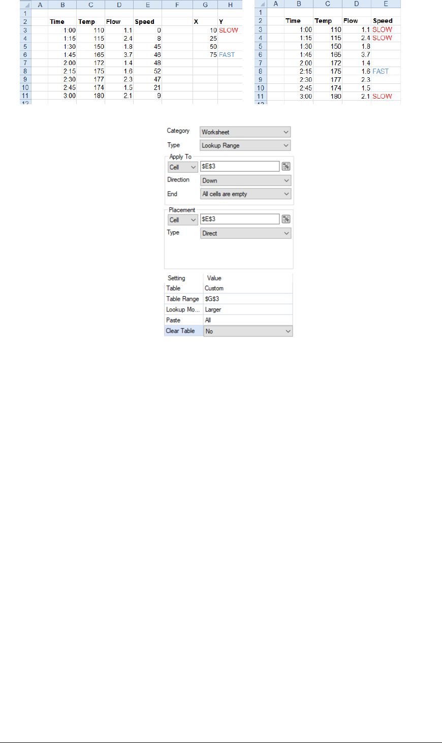
Lookup Range

The Lookup Range function converts values based on a lookup table. Standard Tables such as

On/Off are provided for converting 0/1 values. The lookup table consists of an X and Y column(s)

where the X column is used to for the lookup and the Y column(s) are used for conversion.

The Placement setting determines where the looked-up value is placed in the worksheet. If this

parameter is set the same as the Apply To Cell then the looked-up values overwrite the original values.

Settings

Table

The type of lookup table to use, either a standard table like Yes/No, True/False or On/Off or a

Custom table as defined within a worksheet in the workbook.

Table Range

This is only applicable when Table is set to Custom.

If the range is a single cell or column, that cell/column is treated as the X value of the lookup table

and the column immediately to the right is treated as the Y value.

If the range is a single row with multiple columns, the leftmost column of the range is treated as

the X value of the lookup table and every other column is treated as a Y value. As a simple

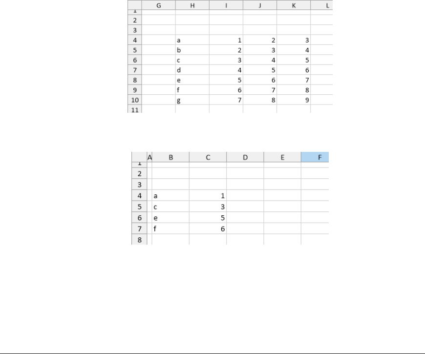
example, consider the following lookup table:

If the Table Range is set to $H$4 or $H$4:$I$4, and is set up so that the Y value appears to the

right of the value in the report the results are:

However, if the Table Range is set to $H$4:$K$4, the results are:

Data Management - 28 -

The number of rows in the table is determined by finding the first empty row in the leftmost (X)

column.

Please note that if the X column is numeric than it must be listed in order either ascending or

descending otherwise the results of the function may not be accurate.

Lookup Mode

• Exact

Only values that match exactly to values in the lookup table are written, anything else is

skipped.

• Smaller

This only applies to ranges where the X value is numeric.

If the values to look up do not match values in the lookup table, the smallest value closest

to the lookup value is considered a match and the Y value is applied.

• Larger

This only applies to ranges where the X value is numeric.

If the values to look up do not match values in the lookup table, the largest value closest

to the lookup value is considered a match and the Y value is applied.

• Closest

This only applies to ranges where the X value is numeric.

If the values to look up do not match values in the lookup table, the closest to the lookup

value is considered a match and the Y value is applied. If there are 2 values in the table

equally distant from the looked-up value, the smaller of the 2 values is considered the

match.

• Interpolated

This only applies to ranges where the X value is numeric.

If the values to look up do not match values in the lookup table, the Y value is

interpolated based on the position in the table.

Paste

This is only applicable when Table is set to Custom.

This determines what is pasted from the Y value(s) of the lookup table when a match is found.

Value pastes just the value from the lookup table, Format just copies the formatting from the

lookup table (no value) and All copies both the formatting and value from the lookup table.

Clear Table

This setting only applies when the Table is set to Custom.

If set to Yes, the lookup table is cleared from the worksheet after the function is complete.

Example

Convert speed values so that values less than 10 show “SLOW” and values greater than 50 show

“FAST”.

Data Management - 29 -

Replace Range

The Replace Range function replaces all occurrences of Find What in the Apply To range with the

Replace With value.

Settings

Find What

The value in the range to be replaced. This can either be a hard coded value (numeric or text), an

XLReporter Name Type or Variable or a combination of both.

To replace any blank cell with a value, leave this setting empty.

Replace With

The value in the range to replace the Find What value with. This can either be a hard coded value

(numeric or text), an XLReporter Name Type or Variable or a combination of both.

To replace a value with a blank, leave this setting empty.

Match Entire Cell

If set to Yes, a value will only be replaced if the entire cell matches the Find What value. If set to

No, the value will be replaced if it is found within a cell.

As a simple example, consider a configuration where Find What is a and Replace With is x. If

the range contains 3 cells with the following values:

abc

If Match Entire Cell is set to Yes, the results would be:

Data Management - 30 -

abc

If No, the results would be:

xbc

Match Case

If set to Yes, when Find What is set to a textual value, case is considered when determining a

match, otherwise it is not.

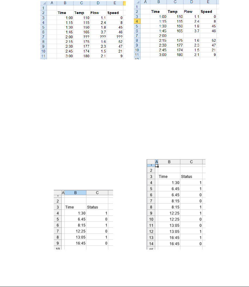
Example

With Find What set to 10 and Replace With set to 2 and Match Entire Cell Contents set to No, a

cell containing “101” is changed to “21”.

Replace all the cells containing ??? with a blank.

Apply To $B$3:$E$3, Down, All cells are empty

Setting

Find What ???

Replace With

Match Entire Cell No

Match Case No

Square Range

The Square Range function inserts additional rows of data into tabular data in order hold the value of

the tag until the next sample.

For example:

Before After

Note that the value at 1:30 is added to the table with the timestamp 6:45 (next sample). This continues

with all the samples in the table.

Data Management - 31 -

When the Square Range management function is applied to charts, it will smooth out the peaks and

valleys which would be shown if the data had not used this function. The most effective chart type to

use for this management function is an XY scatter chart plotting time on the X axis.

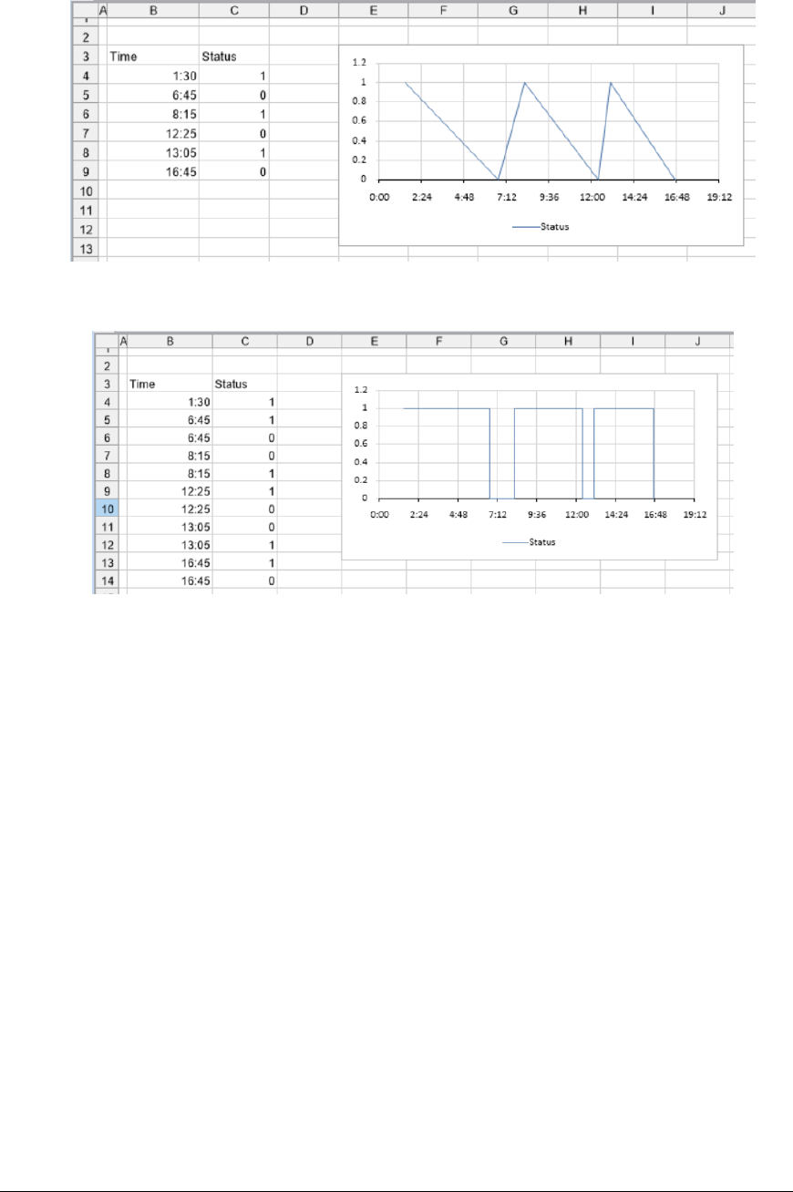
Example

As an example, here is a report with the daily run status of a machine and a chart.

It is hard to determine from the chart the time period when the machine was running and when it was

not. Now, with the Square Range management applied to the data ($B$4:$C$4), the chart is

transformed.

Settings

The Apply To range is the only setting required for this function. This determines the range over

which the function is applied. The timestamp (or whatever is used for the x-axis) is assumed to be the

leftmost column of the range and every other column to the right is assumed to be a data series in the

chart.

Sort Range

The Sort Range function sorts the Apply To range based on sorting conditions.

Settings

Sort By, Then By (2)

The sort conditions to apply to the range. These are defined in the Sort Browser (see below).

Data Management - 32 -

Case Sensitive

When set to Yes, if the column/row to sort contains text, the case is considered when sorting,

otherwise case is not considered.

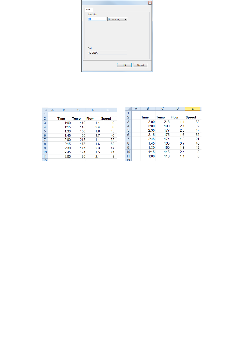
Sort Browser

This browser is used to construct sort conditions. The condition can be entered by selecting it and then

clicking a column/row heading in the worksheet.

Example

Sort the values starting at $B$3:$E$3 by the Temperature in $C$3.

Use the settings:

Apply To $B$3:E$3, Down, All cells are empty

Setting

Sort By $C DESC

Then By

Case Sensitive No

Text Range to Column

The Text Range to Column function splits up the values (numbers or text) in the Apply To range

based on the Delimiter.

The Apply To Range only operates on a single column of data. The Placement defines where the

first split value is placed when the function is executed. Subsequent split values will appear in

columns adjacent to the Placement.

Settings

Delimiter

The text by which to split each cell in the Apply To range. A list of common delimiters is

provided. If the Delimiter required is not listed, it can be manually entered in for the setting.

Data Management - 33 -

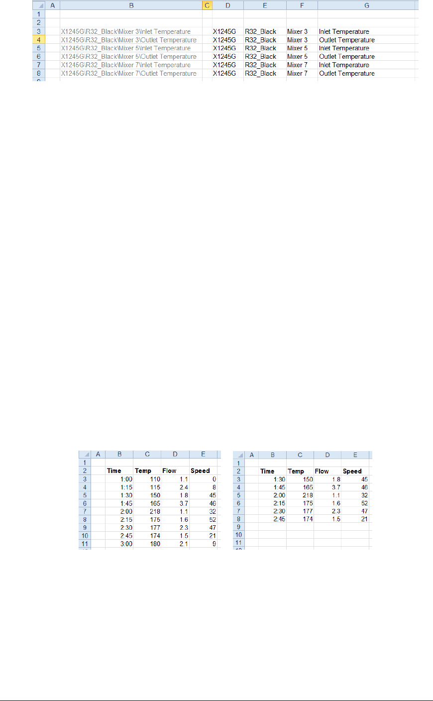
Example

Break the text in the B column based on the backslash (\) delimiter.

Apply To $B$3, Down, All cells are empty

Placement $D$3, Direct

Setting

Delimiter \

Trim Range

The Trim Range function trims the top and/or bottom (or left and/or right depending on Direction) of

the Apply To range until the Condition is satisfied.

Settings

Start

This setting indicates if records are removed from the Top, Bottom or both the Top and Bottom.

Condition

The Condition by which once the values in the range satisfy no other records are removed. This

is specified by using the Filter Browser (see Filter Range).

Case Sensitive

If set to Yes and the Condition is textual, case is considered, otherwise it is not.

Delete Records

If this is set to Yes, the top and/or bottom (depending on Start) removed ranges are physically

deleted from the worksheet causing cells below or to the right of the Apply To range to be shifted

either upwards or leftwards depending on Direction.

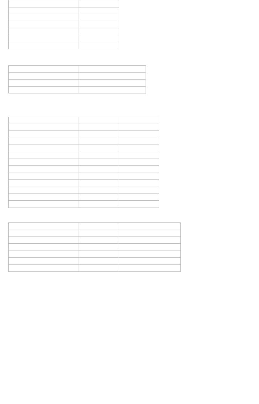
Example

Remove the rows above and below the range until the speed is greater than 10.

Apply To $B$3:E$3, Down, All cells are empty

Setting

Start Top and Bottom

Condition $E > 10

Case Sensitive No

Delete Records No

Data Management - 34 -

Presentation

This set of Data Management functions are used for presentation beyond those provided by the Design

Studio. For example, adding a summary table and chart to report data each time a condition is satisfied,

such as every 8 hours.

Chart Enhancement

The Chart Enhancement function operates on an existing chart to adjust some of its components like

data labels and axes to make the chart more user-friendly. For example, an XY scatter chart

configured over a day showing timestamps can leave a gap on the left and right. Using this function,

the X-axis can be adjusted to span only the day with nothing extra.

If the data series of the chart need to be adjusted for the amount of data to show, use the Chart Range

function under the Worksheet category.

Settings

Chart Name

The name of the chart to apply the function to. The browse button (…) opens a list of every

configured chart within the workbook to select from. The list is in the format:

Chart Name – Sheet!Range of the chart

If a chart is selected in the list, the worksheet for the chart is activated and the range of the chart is

selected to highlight the chart itself.

The chart name is not visible and is typically not set by the user. When a chart is inserted into a

worksheet it is given a default name (Chart X where X is a number that starts at 1). However, if

the worksheet is copied to another sheet, if the default name is left it can be changed on the new

worksheet. To combat this, charts in the template are renamed to a fixed name (xlrX where X is a

number that starts at 1) so that chart names are consistent between worksheets.

Note that only charts configured to worksheets are listed. Charts configured on a Chart Sheet

cannot be used with this function.

Adjust Labels

For each series of the chart, data labels may be turned on so the value of each point is labeled.

However, if the values are textual, the labels show as 0. If you wish to show the textual values for

each point, set this to either In-line or Alternate.

In Line

In-line data labeling displays the label of each point in the same position, e.g., if the data label

of the first point is set above the point, the label for each subsequent point of the series

appears above the point.

Alternate

Alternate data labeling alternates the position of the data label for each point. For example, if

the data label for the first point is above the point, the next is below the point, then above

again and so on. This can be useful if the text of the data labels overlaps with each other.

Anchor Plot Area

If rows or columns are inserted into the report worksheet that causes the chart to expand, it can

leave whitespace at the top or left of the chart because the plot area is moved down or to the right.

This setting can correct this and anchor the plot area to the Left, to the Top or Both. This

eliminates that useless whitespace from the chart.

Data Management - 35 -

Adjust X-Axis

This setting determines if the X-axis of the chart should be adjusted by updating the minimum and

maximum values of the axis. Note that is only valid on charts like XY Scatter where the X-axis is

defined with minimum and maximum values.

First Series means that the minimum and maximum values are derived from the values in the first

series of the chart. If the values are numeric, the minimum is reduced by 1% and the maximum is

increased by 1% before they are applied to the chart.

Custom means that the minimum and maximum values are derived as the minimum and maximum

values from the cell range specified in the Custom Scaling setting.

Custom Scaling

If Adjust X-Axis is set to Custom, this defines the range of cells where the minimum and

maximum values are derived for the X-axis.

Axis Ticks

This setting can be used to fix a number of tick marks for the X and or Y axis. The format of the

setting is X,Y e.g., 5,7 for 5 X axis tick marks and 7 Y axis tick marks. If either is set to 0, the tick

marks for the axis remain unchanged.

Adjust Y-Axis

This setting determines if the Y-axis of the chart should be adjusted by updating the minimum and

maximum values of the axis.

First Series means that the minimum and maximum values are derived from the values in the first

series of the chart. If the values are numeric, the minimum is reduced by 1% and the maximum is

increased by 1% before they are applied to the chart.

Custom means that the minimum and maximum values are derived as the minimum and

maximum values from the cell range specified in the Custom Scaling setting.

Custom Scaling

If Adjust Y-Axis is set to Custom, this defines the range of cells where the minimum and

maximum values are derived for the Y-axis.

Note that the range specified here do not need to be the same ones used in the data series of the

chart.

Example

A daily report template is configured containing an XY scatter chart to graphically display the daily

data. The X axis is configured for the timestamps returned from the group. By default, there is a gap

on the left and right of the chart because the X-axis is more than 1 day.

The Chart Enhancement function can correct this. Assuming the chart is named xlr1, the settings are:

Setting

Chart Name xlr1

Adjust Labels No

Anchor Plot Area None

Adjust X-Axis First Series

Custom Scaling

Axis Ticks 0,0

Adjust Y-Axis No

Custom Scaling

Data Management - 36 -

Cross Tab on State Change

The Cross Tab on State Change function is used to analyze rows of data and cross tabulate (combine)

multiple rows into a single row based on a change in State in a designated column. Consider the

following data:

Date/Time

State

1/1/2020 00:00

1/1/2020 01:00

OFF

1/1/2020 02:00

1/1/2020 03:00

OFF

1/1/2020 04:00

1/1/2020 05:00

OFF

Using this function, the following can be generated:

Start Date/Time

End Date/Time

1/1/2020 00:00

1/1/2020 01:00

1/1/2020 02:00

1/1/2020 03:00

1/1/2020 04:00

1/1/2020 05:00

The data may also have values from multiple sources which must also be considered. This is referred

to as the Key column. Consider the following data:

Date/Time

Pump

State

1/1/2020 00:00

1/1/2020 00:30

1/1/2020 01:00

OFF

1/1/2020 01:30

OFF

1/1/2020 02:00

1/1/2020 02:30

1/1/2020 03:00

OFF

1/1/2020 03:30

OFF

1/1/2020 04:00

1/1/2020 04:30

1/1/2020 05:00

OFF

1/1/2020 05:30

OFF

If the Key column is set to Pump, the following can be generated:

Start Date/Time

Pump

End Date/Time

1/1/2020 00:00

1/1/2020 01:00

1/1/2020 00:30

1/1/2020 01:30

1/1/2020 02:00

1/1/2020 03:00

1/1/2020 02:30

1/1/2020 03:30

1/1/2020 04:00

1/1/2020 05:00

1/1/2020 04:30

1/1/2020 05:30

Settings

Key

This setting defines the column within the range that helps identify what should be considered a

state change. In the example above, the Pump column is used as the Key column so that every

state change of every unique pump is considered separately.

Note that the Key column is not a required setting. It is not needed if all the State values pertain

to the same key.

If the Key is not needed the value of this setting should be left blank. If it is needed it should be

set to the cell in the top row for the appropriate column within the Apply To range.

State

This setting defines the column within the range with the unique state values. This should be set

to the cell in the top row for the appropriate column within the Apply To range.

Data Management - 37 -

State Change

This defines how changes in state are detected.

• Any

Any row where the value in the State column equals Value 1 or Value 2, a state change

has occurred.

If Value 1 and Value 2 are left empty state changes are determined by the first and last

rows where the State value and Key value (if specified) match.

• Distinct

Only the first match of the State column with Value 1 or Value2 is considered a state

change. This means if Value 1 is 0 and there are 5 consecutive rows of 0, only the first is

considered a state change.

• Any Value Change

Any change in value in the State column or Key column (if specified) is considered as

two state changes: the end of the previous state and the beginning of a new one. When

State Change is set to this type, Value 1 and Value 2 are ignored.

Value 1

The value that defines when a new state has been detected. This can be a fixed value or a cell

reference.

Value 2

The value that defines when the exit state has been detected. This can be a fixed value or a cell

reference.

Range 1

This defines the range of cells to copy when a new state has been detected. This should be defined

as a range of cells in the top row of the Apply To range.

This range is pasted to the worksheet based on the Placement cell defined.

Range 2

This defines the range of cells to copy when the exit state has been detected. This should be

defined as a range of cells in the top row of the Apply To range.

Range 2 Placement

This setting determines how Range 2 is written to the worksheet.

• At End

Range 2 is placed directly to the right of Range 1.

• Append

Range 2 is appended to the first empty cell at or to the right of the Placement column.

• Insert At Start

Range 2 is inserted at the Placement column pushing the Range 1 data to the right.

• Insert At End

Range 2 is inserted immediately to the right of the end of the Range 1 data pushing

anything to the right outwards.

Mechanics

State Change is Any or Distinct

When the State Change is Any or Distinct, if the State value equals Value 1, the range specified

in Range 1 is copied to the Placement cell and the Key value (if specified) is retained. If the

State value equals Value 2, the range specified in Range 2 is copied to the Placement area. If the

Key column is specified, Range 2 is pasted to the row corresponding to the Key, otherwise it is

pasted to the row of the last Value 1 state change.

Data Management - 38 -

If State Change is Any and Value 1 and Value 2 are left blank, each unique set of State and Key

(if specified) values are determined. Range 1 is copied from the first row containing the set and

Range 2 is copied from the last row containing the set.

State Change is Any Value Change

When the State Change is Any Value Change when any state change is detected, the range

specified in Range 2 is copied and pasted to the row of the previous state change. Then the range

specified in Range 1 is copied and pasted to the new row in the Placement area.

When data is copied to the Placement area, if the Placement Cell has no formatting applied to it, the

format in the Apply To range is copied along with the values, otherwise only the values are pasted.

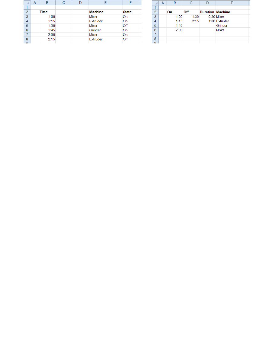
Example

Calculate runtimes from an event log of machine starts/stops.

Use the settings (the duration is a formula):

Apply To $B$3:F$3, Down, All cells are empty

Setting

Key $E$3

State $F$3

State Change Any

Value 1 On

Value 2 Off

Range 1 B3:E3

Range 2 B3

Range 2 Placement Append

Insert Into Range

The Insert Into Range function takes a Collection (a range of cells containing items such as formulas

and charts) and inserts them above, below and/or within the Apply To range. The function can be

used to insert subtotals and charts into a range of data.

Settings

Top Collection

This setting is a range of cells containing all the labels, formatting, formulas, and charts to insert at

the top of each determined range (as defined by Insert Mode). This range must be on the same

worksheet as the Apply To range.

Any charts or formulas within the collection that refer to data in the Apply To range should only

reference the top row within the range. When the Collection is inserted, all of these cell

references are automatically adjusted to the amount of data in the range.

Bottom Collection

This setting is a range of cells containing all the labels, formatting, formulas, and charts to insert at

the bottom of each determined range (as defined by Insert Mode). This range must be on the

same worksheet as the Apply To range.

Any charts or formulas within the collection that refer to data in the Apply To range should only

reference the top row within the range. When the Collection is inserted, all of these cell

references are automatically adjusted to the amount of data in the range.

Data Management - 39 -

Paste

This defines what is pasted from the Collection(s) to the range. This can be set to just copy the

Values, just the Fomulas or All to copy everything in the Collection(s) including all formatting

configured.

Insert Mode

This defines how the Collection(s) are inserted into the range.

All means that the Top Collection (if defined) is inserted at the very top of the Apply To range

and the Bottom Collection (if defined) is inserted at the very bottom of the Apply To range.

Column Change means that at every change in value of a specified Column (see below) the

Collection(s) are inserted into the range.

Column

If Insert Mode is set to Column Change, this setting defines the column in the range to monitor

for a change in value. The setting must be set to a column reference, e.g., $B for the B column.

Add Grouping

When set to Yes, every Collection inserted into the range will have an outline defined for it within

the worksheet. The outline appears to the left of the row labels and can be used to show or hide

the rows within it.

Initial State

If Add Grouping set to Yes this setting defines the initial state of the group outline, either

Expanded or Collapsed.

Clear Collection

If set to Yes, after the function is complete the Collection range(s) are cleared from the worksheet.

Example

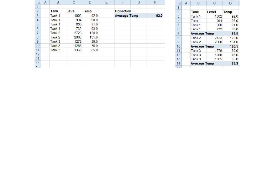
Add a subtotal showing the average temperature of each tank.

The collection contains an average in H3 = AVERAGE(D3)

Apply To $B$3:D$3, Down, All cells are empty

Setting

Top Collection

Bottom Collection $F$3:$H$3

Paste All

Insert Mode Column Change

Column $B

Add Grouping No

Initial State Expanded

Clear Collection No

Data Management - 40 -

List from Bitmask

PLC integers used as bitmasks are useful for holding information by assigning each bit to a specific

requirement. For example, a 16-bit integer could represent 16 different states of the process.

This function expands an integer into a list where each row represents a bit of the integer that is “set”.

The expansion can also include other values.

Example

Suppose that at the end of a machine cycle, the date/time, operator, and an integer bitmask is saved to

the report (the bitmask here could represent certain actions that the operator performed during the

cycle.

Result

Going a step further, if a Lookup Range function is applied, the numeric in the list can be converted to

a readable text string.

Setting

Outline Range

The Outline Range function removes repeating values in rows or columns (depending on Direction)

in the Apply To range. The function removes repeats on the first column. It then removes repeats on

the next column only if there was a repeat on the previous column. This continues until the range is

completed.

Settings

Match Case

If set to Yes, when comparing textual values for repeats, the case is considered, otherwise it is not.

Delete Empty

If set to Yes, if the empty rows or columns are left in the Apply To range, the rows or columns are

deleted from the range. Otherwise, empty rows or columns will remain in the range.

Example

Remove repeating values starting on row 3.

Data Management - 41 -

Apply To $B$3:E$3, Down, All cells are empty

Setting

Match Case No

Delete Empty No

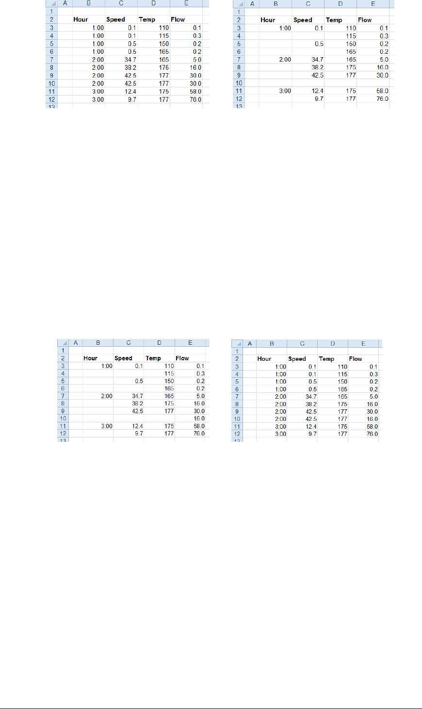
Propagate Range

The Propagate Range function propagates the value and format of non-empty cells down (or across)

into empty cells within the Apply To range. This function can be used to handle sparse data or to

produce a contiguous row or column of data for a chart.

Settings

Mode

The mode in which the data is propagated to empty cells. The Staircase mode copies the value

from the last non-empty cell to the empty cells.

Example

Fill empty cells starting on row 3.

Apply To $B$3:E$3, Down, All cells are empty

Setting

Mode Staircase

Stack Range

The Stack Range function stacks groups of columns in the Apply To range by placing the leftmost

column of the group in the Placement and leaving the remaining columns in place. This function can

be used to combine data logged at different intervals into a single table with sparse data.

This can be very useful if the report has multiple data sources and you want to combine that data

together into a single table to see what happened at what time. It is also useful if multiple data groups

must be used to retrieve all the data required for the report.

Note that the Apply To range does not need to include the first group since that is already correctly

positioned.

Data Management - 42 -

Settings

Rows In Header

The number of rows above the Apply To range to consider as headers. When the leftmost column

of the group is stacked, the headers row(s) for that column are removed.

Column Group Count

The number of columns for a group.

Sort

This indicates whether or not to sort the resultant range based on the values in the column of the

Placement. None indicates no sorting will be done, while Ascending and Descending apply a sort

to the range.

If the results are sorted, duplicate values in the Placement are combined together to form a single

row.

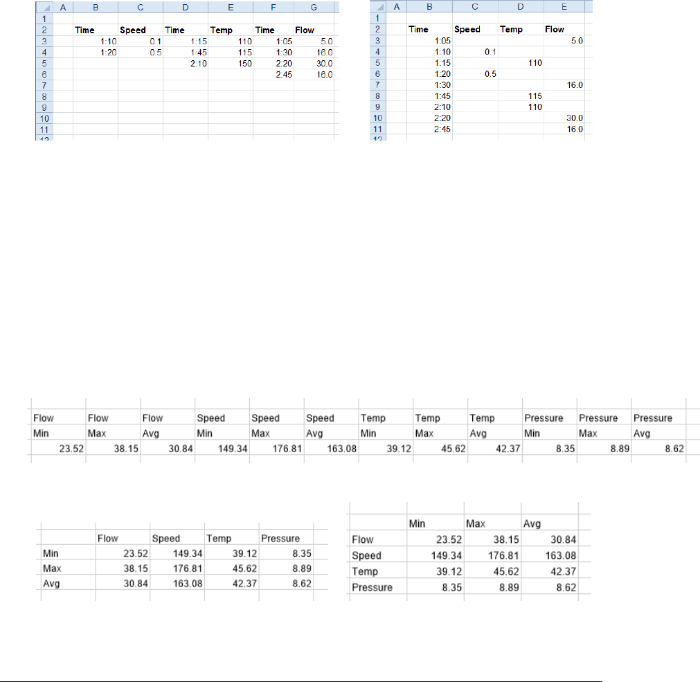
Example

Combine raw data for Speed, Temperature and Flow into a table with a common timestamp.

Apply To $D$3:G$3, Down, All cells are empty

Placement $B$3

Settings

Rows In Header 1

Column Group Count 2

Sort Ascending

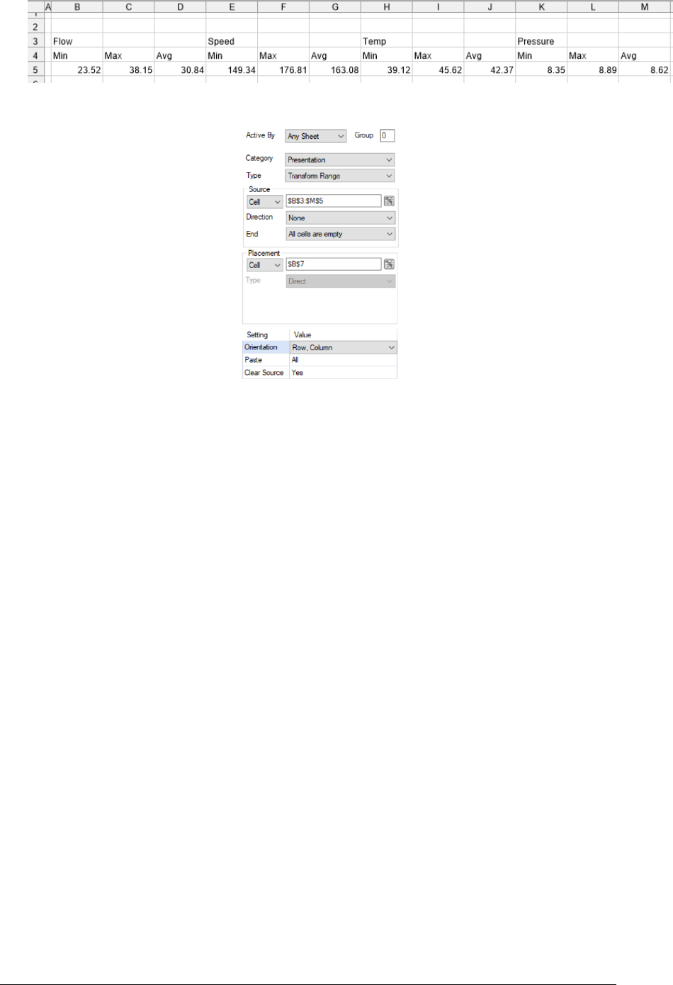
Transform Range

The Transform Range function takes a range consisting of two rows of headings and one row of data

and transforms this to a summary table.

For example, suppose the values in the report are displayed as follows (typical format from a history

group):

Using this function, this data can be shown as a summary table in either of the two styles:

The transformation takes the top two rows and treats them as either the column or row captions. The

third row is used as the data for the summary table.

Data Management - 43 -

If the Source does not contain 3 rows then this function does nothing, more than 3 rows then the first 3

rows are considered. If there are empty cells within the headings of the Source range, it assumes the

text of the cell to the left. For example, if the Source range is:

The headings in $C$3 and $D$3 are treated as Flow, $F$3 and $G$3 are Speed and so on.

The Placement can be set to a cell within the Source range.

Settings

Orientation

This setting determines the orientation of the summary table.

• Column, Row

The first row of the Source becomes the \ column headings and the second row becomes

the row headings of the summary table.

• Row, Column

The first row of the Source becomes the row headings and the second row becomes the

column headings of the summary table.

Paste

The elements from the Source (e.g., formats) that are applied to the summary table. This applies

both to the row and column headers as well as the data.

Clear Source

If set to Yes, the Source range is cleared, otherwise it is left in the sheet.

Example

A user can select up to ten tags from their historian to get the minimum, maximum and average over a

specified time period. The report is to show each selected tag as a row with the minimum, maximum

and average shown as three columns.

The history data group provides the data which has the Columns and Time Period tabs configured as

follows:

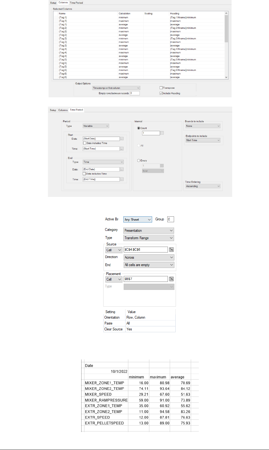
Data Management - 44 -

This group is connected to cell $B$4 in the template. The Transform Range management function is

set up as:

Note that the Source starts on column C since the timestamp is in column B. It also acounts for the

user selecting a variable number of tags.

The summary table produced for the report will look like:

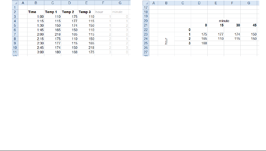
Data Management - 45 -

2D Transformation

The 2D Transformation function works on a table of three columns where one column is the X

coordinate, one column is the Y coordinate, and the last column is the value to create a new table of

values based on the coordinates.

Settings

Row Offset

The cell that contains the X coordinate for transformation. This cell should be in the same row as

the top row in the Base range and the column should be contained within the Base range.

Row Origin

The origin point for the Row Offset values. Typically, this is set to 0 but in cases where the

offsets are non-zero this can compensate. For example, if the Row Offset values are the days of

the month (1-31) this can be set to 1.

Column Offset

The cell that contains the Y coordinate for transformation. This cell should be in the same row as

the top row in the Base range and the column should be contained within the Base range.

Column Origin

The origin point for the Column Offset values. Typically, this is set to 0 but in cases where the

offsets are non-zero this can compensate. For example, if the Column Offset values are the days

of the month (1-31) this can be set to 1.

Data Range

This setting defines the range of data copied from the Base range. This should be one or more

columns from the top row of the Base range.

Paste

This setting defines what is pasted from the Data Range to the Placement for every row.

Clear Data

If set to Yes or Yes (Extended), all the data from Base range is cleared. Yes (Extended) also clears

any headers above the Base range.

Example

Display temperature 2 in in a minute/hour display.

Note the two additional columns hour and minute using functions which are used to detemine the

placement of the temperature value (in practice these would be hidden).

Base $C$3:E$3, Down, All cells are empty

Placement $D$22

Settings

Row Offset $F$3

Row Origin 0

Column Offset $G$3

Column Origin 0

Data Management - 46 -

Data Range $D$3

Paste All

Clear Data No

Value Limit Range

The Value Limit Range function filters or color codes the Apply To range based on the Low Limit

and/or High Limit specified.

Settings

Low Limit

The value by which if any value in any cell within the Apply To range is less than or equal to, that

value is considered outside the limits.

This can be specified as a fixed number or a cell reference.

High Limit

The value by which if any value in any cell within the Apply To range is greater than or equal to,

that value is considered outside the limits.

This can be specified as a fixed number or a cell reference.

Show Values

This setting defines what to show after the function has executed.

• All

All values in the Apply To range are displayed with values outside the limits formatted as

defined below.

• Between Limits

Only values between the Low Limit and High Limit defined are shown in the Apply To

range. Values outside the limits are cleared.

• Outside Limits

Only values outside the Low Limit and High Limit defined are shown in the Apply To

range. Values within the limits are cleared.

Low Format

The background color for any value less than or equal to the Low Limit. This can either be a

specific color listed or a numeric color in the R,G,B format. For example, a gray background

could be specified as 128,128,128.

Between Format

The background color for any value between the Low Limit and High Limit. This can either be a

specific color listed or a numeric color in the R,G,B format. For example, a gray background

could be specified as 128,128,128.

High Format

The background color for any value greater than or equal to the High Limit. This can either be a

specific color listed or a numeric color in the R,G,B format. For example, a gray background

could be specified as 128,128,128.

Delete Empty Rows

This setting only applies if Show Values is set to Between Limits or Outside Limits.

If set to Yes, if the function results in completely empty rows within the Apply To range, the row

is deleted from the range. Otherwise, empty rows will remain in the Apply To range.

Extend Columns

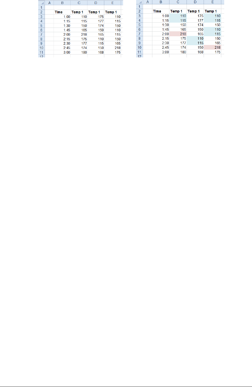
Data Management - 47 -

If Delete Empty Rows is set to Yes, this is the number of columns to extend to the left and right to

include when deleting the rows. For example, the extend the range by 1 column to the left and 2

to the right, set this to 1,2.

Example

Color code temperatures below 140 and greater than 200.

Settings

Apply To $C$3:E$3, Down, All cells are empty

Setting

Low Limit 140

High Limit 200

Show Values All

Low Format Sky Blue

Between Format None

High Format Light Red

Delete Empty Rows No

Extend Columns 0,0

Weave Into Range

The Weave Into Range function weaves a Collection range into the Apply To range, preserving the

formatting of each if requested.

The function compares each value in leftmost column of the Collection range to the leftmost column

of the Apply To range. When a match is found, the row in the Collection range is placed into the

Apply To range based on the Weave Mode setting. If a match is not found, then the location of the

closest match is determined. Note that the values of the leftmost column of the Apply To range must

be ordered.

Settings

Weave Mode

This setting determines how the values from the Collection range are written to the Apply To

range.

• Column Insert

For every row in the Collection range, a row is inserted into the Apply To range

regardless as to whether the values in the leftmost column of both ranges match.

The value of the leftmost cell of the Collection range is copied to the leftmost cell of the

inserted row in the Apply To range. The remaining values in the Collection range are

copied to the right edge of the Apply To range.

• Row Append

For every row in the Collection range, if the value in the leftmost column matches the

value in the leftmost column of the Apply To range, the values from the second column

outward in the Collection range are copied and pasted to the right edge of the Apply To

range.

If no match is found a row is inserted into the Apply To range, the value from the

leftmost column in the Collection range is copied and pasted to the leftmost column of

the Apply To range. The remaining columns in the Collection range are copied and

pasted to the right edge of the Apply To range.

Data Management - 48 -

• Replace Blanks and Errors

The values in the Collection range are only copied over blanks and errors in the Apply

To range.

This is most useful when a data connector does not provide a Secondary Server and

there are redundant data servers available to retrieve data from and the report should use

data from the secondary server if data from the primary is not available.

In this scenario, two data connections are added into a template. These connections are

identical except one is connected to the primary server and the other connected to the

secondary. The Apply To range of the Weave Into Range is configured for the range

where the primary server data connection is configured and the Collection range for the

secondary server. If any values are missing from the primary server connection or return

an error symbol (???, ###, @@@ or !!!), the values from the Collection range are woven

into the Apply To range.

Use Collection Format

If set to Yes when values are copied from the Collection to the Apply To range, the format from

the Collection is pasted with it. Otherwise, the formatting of the Apply To range is used.

Add Grouping

Grouping allows rows or columns to be shown and hidden in a worksheet. When grouping is set

on a number or rows or columns a button is added to the left or top that allows you to expand or

contract the rows or columns on the sheet. This can be added automatically to the rows or

columns of data woven in from the Collection range so that data can be easily shown or hidden

within the Apply To data by setting Add Grouping to Yes.

Initial State

If Add Grouping is set to Yes, this setting determines if the Collection data is Expanded or

Collapsed when the report is initially generated.

Clear Collection

This setting determines if the Collection range is cleared after the function is complete.

• None

The Collection range is not cleared.

• All

The Collection range is cleared including any applied formatting.

• All (extended)

The Collection range is first extended upwards to detect any headings, then the range is

cleared including any applied formatting.

• Contents

The contents of the Collection range are cleared. Any formatting applied will remain.

• Contents (preserve leftmost column)

The contents of the Collection range with the exception of the leftmost column are

cleared. Any formatting applied will remain.

Example

Combine alarm data into process data.

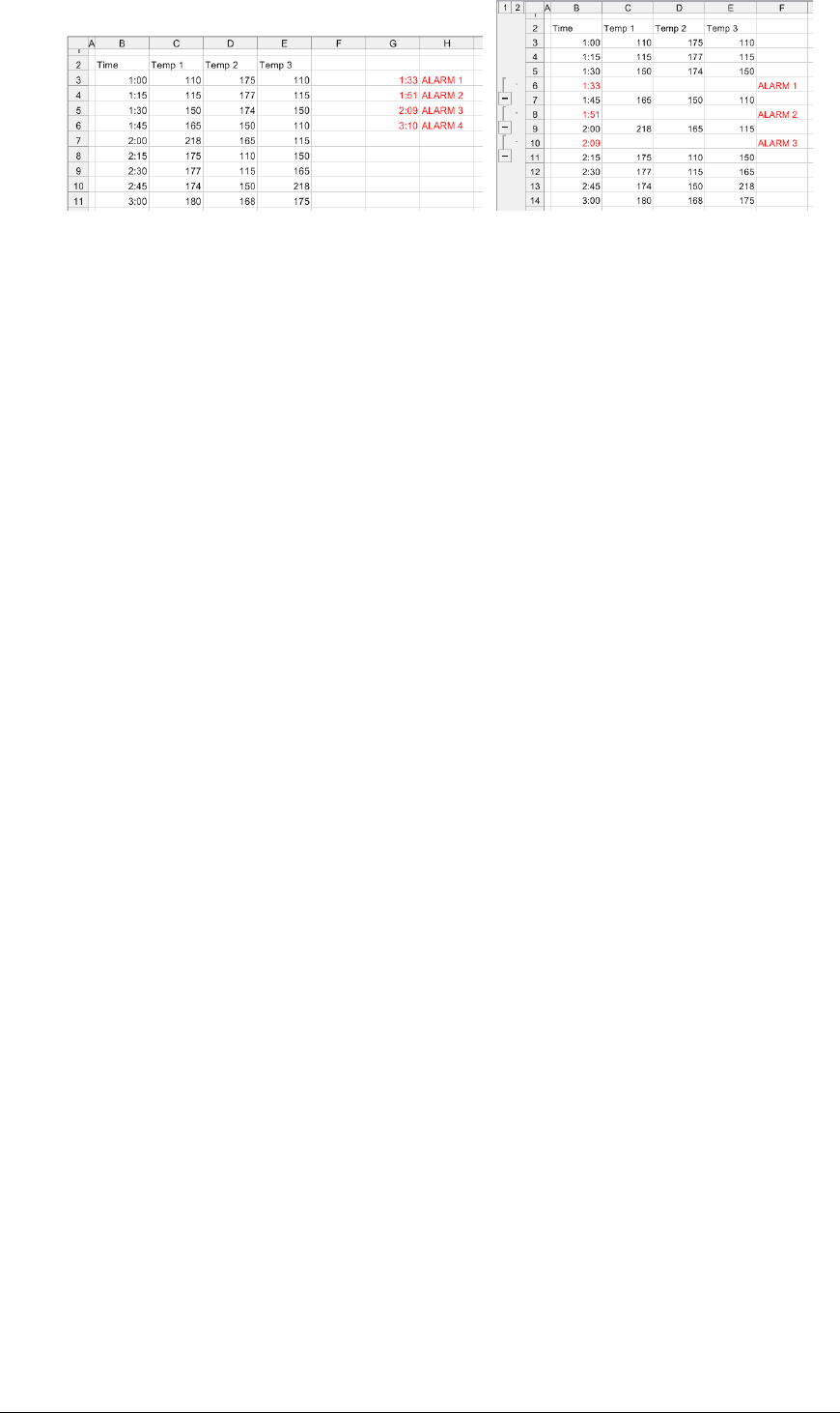
Data Management - 49 -

Settings

Apply To $B$3:E$3, Down, All cells are empty

Collection $G$3:H$3

Settings

Weave Mode Column Insert

Use Collection Format Yes

Add Grouping Yes

Initial State Expanded

Clear Collection All

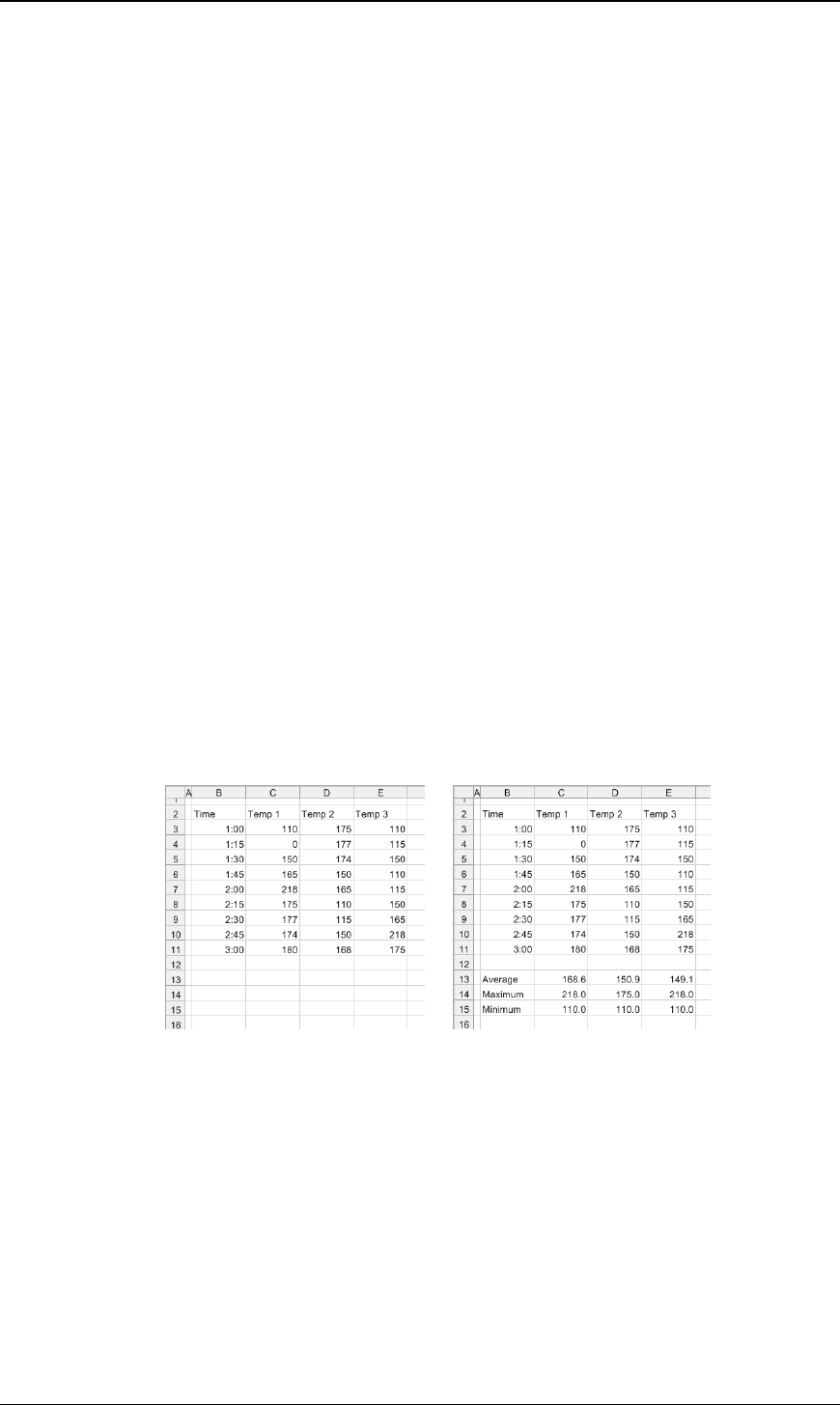
Data Management - 50 -

Analysis

This set of Data Management functions are used for statistical analysis.

Conditional Summary

The Conditional Summary function generates summary values from the Base range using the

Calculation(s) specified and places the results as a table at the Placement.

Settings

Condition

The Condition to apply to every column (or row depending on Direction) to derive the

Calculation(s) specified).

This is specified by using the Filter Browser (see Filter Range).

Calculation (up to 5)

The Calculation to apply to every column (or row depending on direction) in the Base range.

If the Direction is Down or None, each Calculation appears as a row in the Placement whereas if

Direction is Across each Calculation appears as a column in the Placement.

Add Labels

If set to Yes and the Direction is Down or None, labels for each Calculation appear to the left of

the data. If the Direction is Across, labels appear above the data.

Case Sensitive

If the Condition is textual and case is important, set Case Sensitive to Yes.

Example

Calculate the average, maximum and minimum.

Use the settings:

Base $C$3:E$3, Down, All cells are empty

Placement $C$13

Setting

Condition $C > 0

Calculation Average

Calculation Maximum

Calculation Minimum

Calculation None

Add Labels Yes

Case Sensitive No

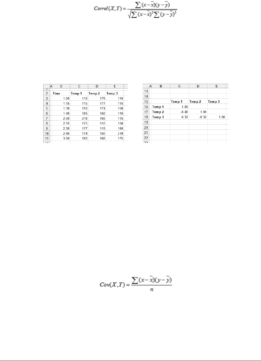
Data Management - 51 -

Correlation

The Correlation function examines the measurements in the Base range and places their correlation in

a table at the Placement. The table displays each combination of column pairs.

Correlation determines whether the two measurements tend to move together i.e., large values of one

tend to be associated with large values of the other (positive correlation), small values of one tend to be

associated with large values of the other (negative correlation) or the value are unrelated (correlation

near 0). Correlation coefficient is scaled to lie between -1 and +1 inclusive.

The equation for the correlation coefficient is:

Settings

Place Formula

If set to Yes, the Correlation formulas are left in the Placement. If set to No, only the values

appear in the Placement.

Example

Determine the correlation coefficients of temperature data.

Temp 1 and Temp 3 are in positive correlation

Base $C$3:E$3, Down, All cells are empty

Placement $C$16

Setting

Place Formulas No

Covariance

The Covariance function examines the measurements in the Base range and places their covariance in

a table at the Placement. The table displays each combination of column pairs.

Covariance determines whether the two measurements tend to move together i.e., large values of one

tend to be associated with large values of the other (positive covariance), small values of one tend to be

associated with large values of the other (negative covariance) or the value are unrelated (covariance

near 0). Covariance is not scaled.

The equation for the covariance coefficient is:

Settings

Place Formula

If set to Yes, the Covariance formulas are left in the Placement. If set to No, only the values

appear in the Placement.

Example

Determine the covariance of temperature data.

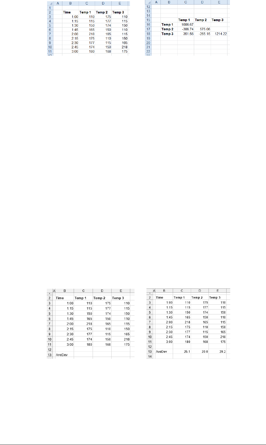
Data Management - 52 -

Base $C$3:E$3, Down, All cells are empty

Placement $C$16

Setting

Place Formulas No

Descriptive Formulas

The Descriptive Formulas function generates values from the Base range using the Formula(s)

specified and places the results as a table at the Placement.

Settings

Formula (up to 6)

The formula to apply to every column (or row depending on Direction) in the Base range. This

can be any formula supported by Excel with # used in place of the cell reference for the column

(or row).

For example, to count all the values in each column that are greater than 0, set Formula to

=COUNTIF(#,”>0”)

Add Labels

If set to Yes and the Direction is Down or None, labels appear to the left of the data. If the

Direction is Across, labels appear above the data. Labels are derived from the formula name.

Place Formula

If set to Yes, the formulas are left in the Placement. If set to No, only the values appear in the

Placement.

Example

Calculate the average of the absolute deviations of temperature.

Base $C$3:E$3, Down, All cells are empty

Placement $C$13

Setting

Formula =AveDev(#)

Formula

Data Management - 53 -

Formula

Add Labels No

Place Formula No

Descriptive Statistics

The Descriptive Statistics function generates statistical values from the Base range using the

Statistic(s) specified and places the results as a table at the Placement.

Settings

Statistic (up to 6)

The statistic to derive for each column (or row depending on the Direction). The following are

available:

• Average

The arithmetic mean.

• Count

A count of non-empty cells

• Kurtosis

Characterizes the relative peakness or flatness of a distribution compared with the normal

distribution. Positive indicates a relatively peaked distribution while negative indicates a

relatively flat distribution

• Maximum

The largest value

• Median

The middle value

• Minimum

The smallest value

• Mode

The most frequently occurring value

• Range

The difference between the maximum and the minimum,

• Sample Variance

The variance

• Skewness

Characterizes the degree of asymmetry of a distribution around its mean. Positive

skewness indicates a distribution with an asymmetric tail extending toward more positive

values. Negative skewness indicates a distribution with an asymmetric tail extending

toward more negative values.

• Standard Deviation

The standard deviation is a measure of how widely values are dispersed from the average

value (the mean).

• Standard Error

The Standard error of the mean.

• Total

The total.

Add Labels

If set to Yes and the Direction is Down or None, labels appear to the left of the data.

Place Formula

If set to Yes, the formulas are left in the Placement. If set to No, only the values appear in the

Placement.

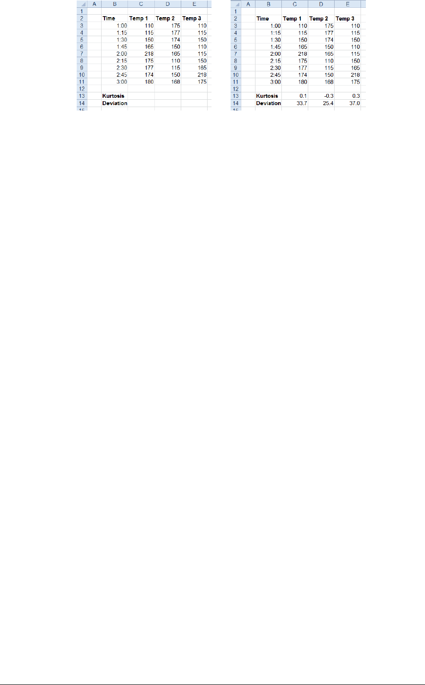
Data Management - 54 -

Example

Calculate the kurtosis and standard deviation of temperatures.

Base $C$3:E$3, Down, All cells are empty

Placement $C$13

Setting

Statistic Kurtosis

Statistic Standard Deviation

Statistic

Add Labels No

Place Formula No

Exponential Smoothing

The Exponential Smoothing function is used to smooth out irregularities (peaks and valleys) to easily

recognize trends.

The function uses the smoothing constant (α) which is associated with the Damping Factor (1- α).

The larger the damping factor, the more the peaks and valleys are smoothed out. The smaller the

damping factor, the closer the smoothed values are to the actual data points.

Settings

Damping Factor

The smoothing constant to apply. This can be a fixed number or a cell reference which contains

the Damping Factor to apply.

Standard Error

If set to Yes, a Standard Error column is added to the Placement.

Place Formula

If set to Yes, the formulas for the smoothing as well as the Standard Error (if included) remain in

the Placement. If set to No, only values appear in the Placement.

Empty Cell Padding

If set to Yes, the values written to the Placement Cell start one row down or one column to the

right (depending on Direction). Otherwise, values start at the Placement cell itself.

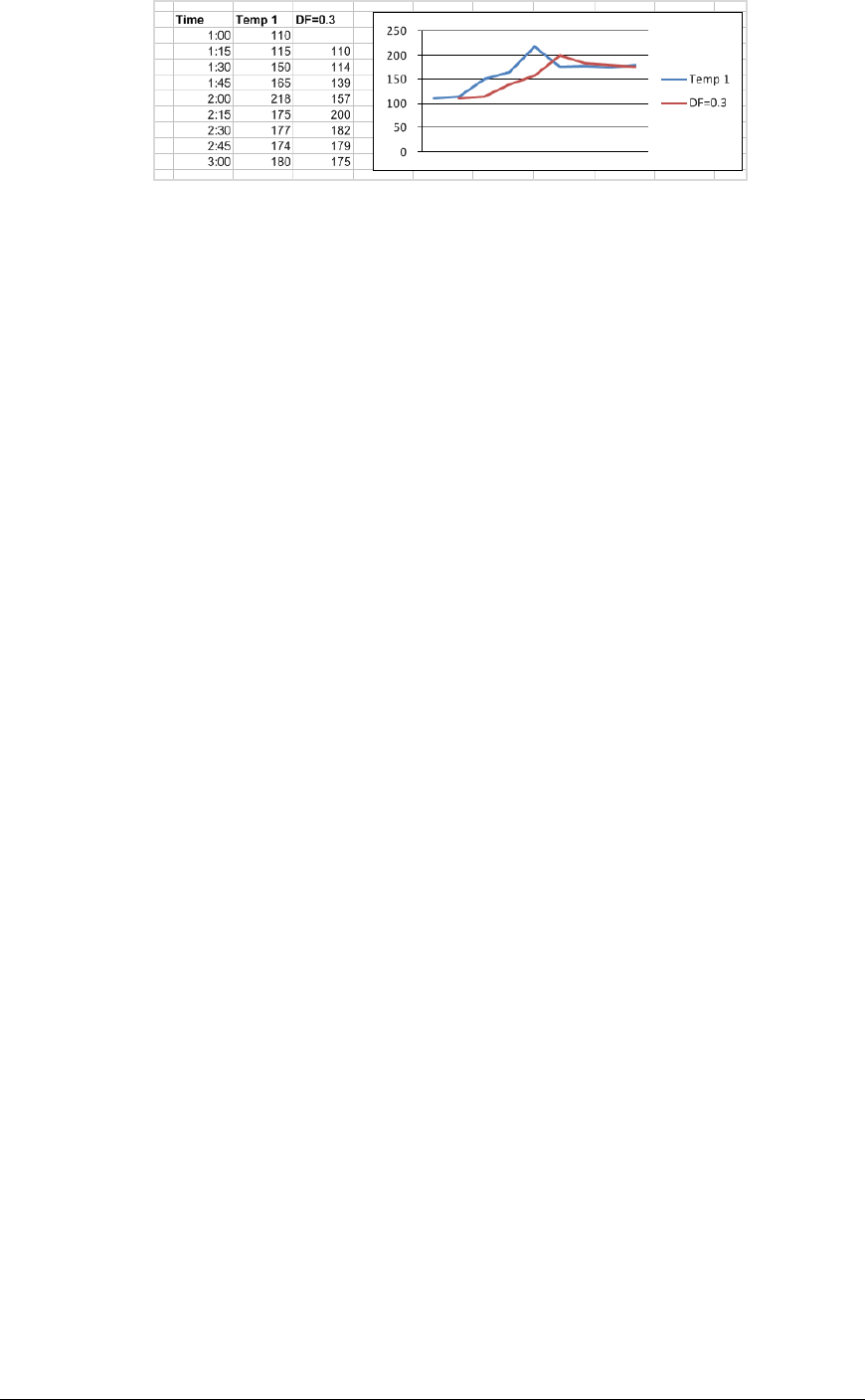
Data Management - 55 -

Example

Smooth the trend of a temperature

Base $C$3, Down, All cells are empty

Placement $D$3

Setting

Damping Factor 0.3

Standard Error No

Place Formula No

Empty Cell Padding Yes

Histogram

The Histogram function calculates individual and cumulative frequencies for a cell range of data and

data bins. It also generates data for the number of occurrences of a value in a data set.

Settings

Bin Range

The bins are defined by setting the Bin Range.

If the Bin Range is 0, every unique value in the Base range is a bin. This can be used to a get a

frequency of every unique value in a range.

If the Bin Range is greater than zero, then the bins are equally spaced between the minimum and

maximum values of the Base.

If the Bin Range is a cell range, the cell values in the range are used as bins. When specified as a

cell range the range should only be 1 column wide.

Pareto

If set to Yes, the resultant table is shown in descending order of frequency.

If the Bin Range is a cell reference, is on the same worksheet and starts on the same row as the

Placement cell, the resultant table is expanded to include the Bin Range as well as any other

columns in between.

For example, if the Bin Range is $B$4:$B$9 and the Placement is $D$4, if Pareto is set to Yes,

the resultant table to sort in descending order is $B$4:$D$9.

Place Formula

If set to Yes, the formulas remain in the Placement. If set to No, only values appear in the

Placement.

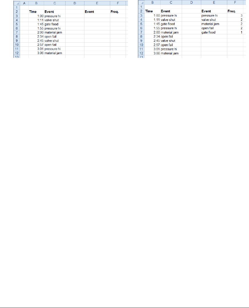
Data Management - 56 -

Calculation (up to 4)

In addition to frequency distribution, additional Calculation(s) can be selected which will appear

as additional columns to the right of the Placement. The following are available:

• Percentage

This calculates the percentage of frequency for each bin.

• Cumulative Percentage

This calculates the cumulative percentage of frequency for each bin.

• Rank

This calculates the rank of frequency for each bin.

• Percentile

This calculates the percentage rank (percentile) of frequency for each bin.

Example

Show the frequency of process events in order of occurrence.

Base $C$3, Down, All cells are empty

Placement $E$3

Setting

Bin Range 0

Pareto Yes

Place Formula No

Calculation

Moving Average

The Moving Average function projects values in the forecast period, based on the average value of the

variable over a specific number of preceding periods. A moving average provides trend information

that a simple average would mask. Use this to forecast sales, inventory, or other trends.

Settings

Interval

The number of preceding values to consider for the Moving Average. This can be a fixed number

or a cell reference.

Standard Error

If set to Yes, a Standard Error column is added to the Placement.

Place Formula

If set to Yes, the formulas for the average as well as the Standard Error (if included) remain in

the Placement. If set to No, only values appear in the Placement.

Empty Cell Padding

If set to Yes, the values written to the Placement Cell start at the end of the first interval down or

to the right (depending on Direction). Otherwise, values start at the Placement cell itself.

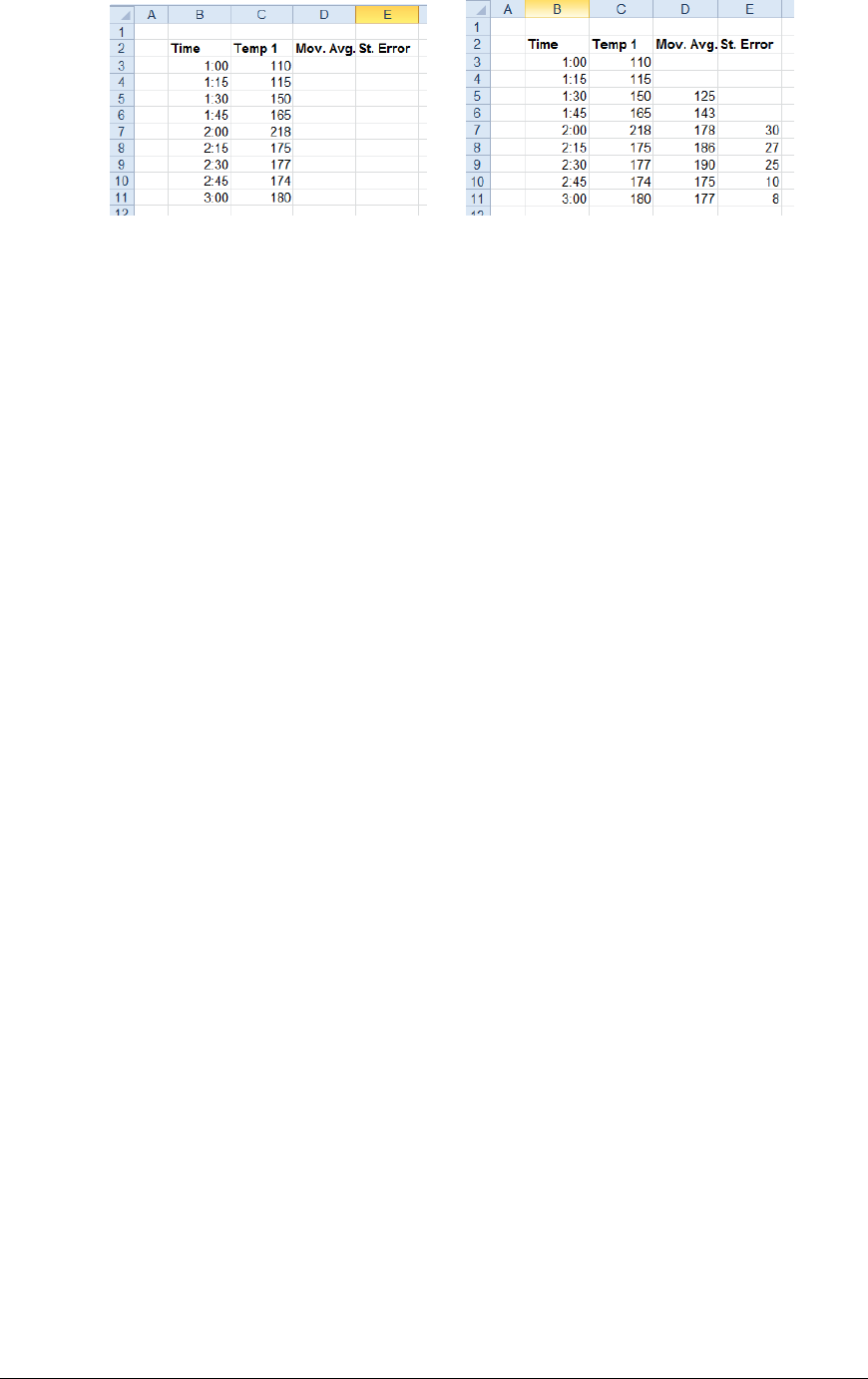
Data Management - 57 -

Example

Show the moving average and standard error of a temperature.

Base $C$3, Down, All cells are empty

Placement $D$3

Setting

Interval 3

Standard Error No

Place Formula No

Empty Cell Padding Yes

Summarize Range

The Summarize Range management function is used to summarize a table of raw data based on an

Interval specified. For example, if the worksheet contains 1 minute raw samples over day, this

function can derive hourly calculations for those samples.

The Formulas for the first “set” of calculations are configured on the sheet and from there the

subsequent formulas are derived and added to the report. If you do not require a summary formula like

Average or Max, but rather, want to show the value every X number of seconds, this function can do

that. For the “formula”, enter the top cell you want to show surrounded by parenthesis, e.g., (B3).

This can also be used to show the timestamp at the beginning of each Interval.

Settings

Formulas

The range of cells containing the Formulas to use for the function.

Interval

The Interval to apply to the cell references in the Formulas to derive the summaries. This can be

a hard coded value or a cell reference.

Place Formula

If set to Yes the formulas remain in the worksheet, otherwise the formulas are removed so that

only the values remain.

Apply Formatting

If set to All, the formatting applied to the Formulas range is applied to all other rows (or

columns). Otherwise, no formatting is applied.

Example

Show the hourly average of 2 temperatures from 1 minute raw data.

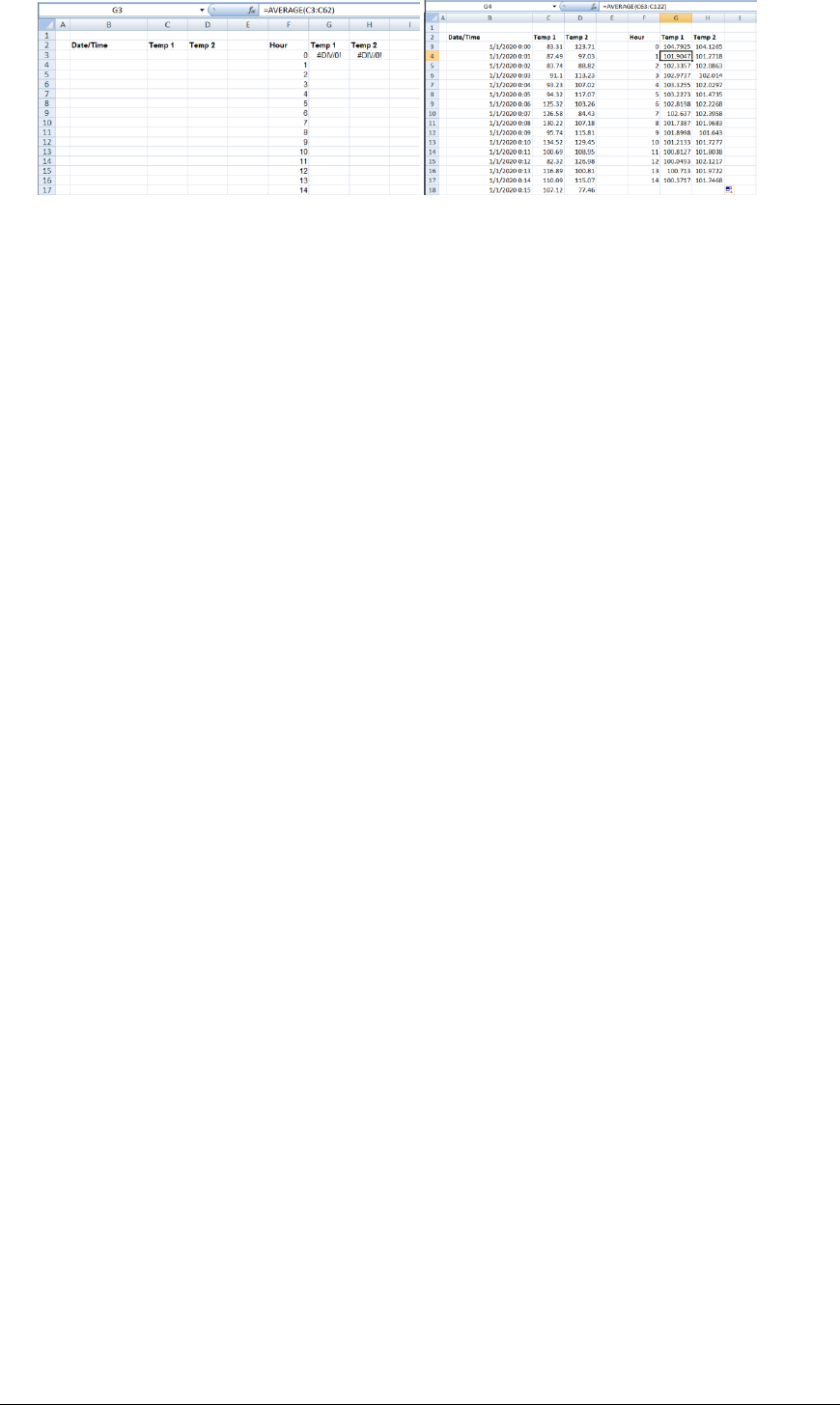
Data Management - 58 -

Base $B$3:$D$3, Down, All cells are empty

Setting

Formulas $G$3:$H$3

Interval 60

Place Formula Yes

Apply Formatting All

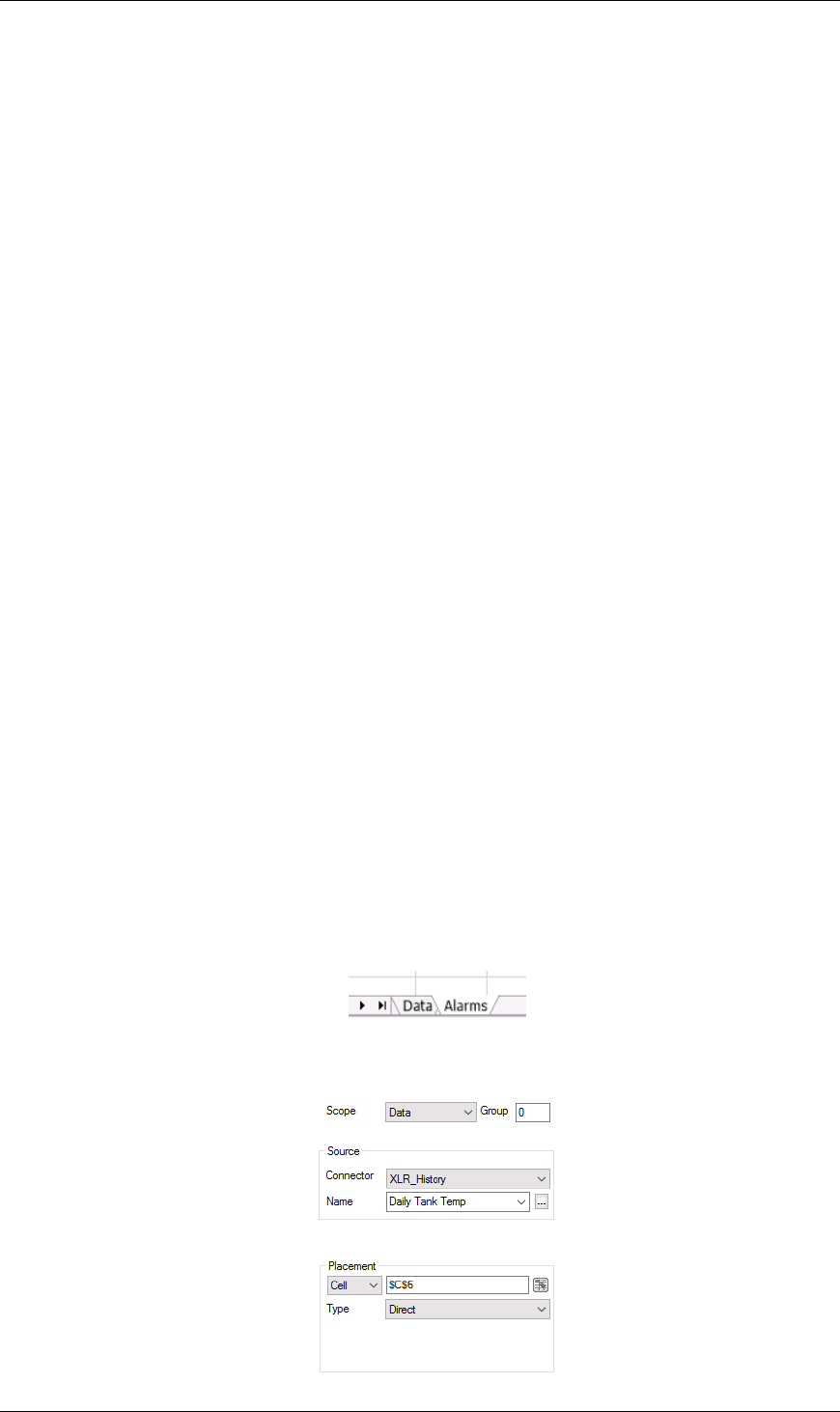
Data Management - 59 -

Cell Action

This set of Data Management functions provide ways to trigger actions based on values in cells in the

report. For example, only when the value of a cell is out of tolerance, a specific group of connections

is updated in the report.

By Value

The By Value function evaluates the Criteria specified and if it is satisfied, triggers the Action

specified.

Setting

Action

The Action to trigger if the Criteria is satisfied. This can be UpdateBook, UpdateSheet,

UpdateGroupBook or UpdateGroupSheet.

Worksheet

If the Action is set to UpdateSheet or UpdateGroupSheet, the Worksheet must be set to the name

of a worksheet in the template.

Group

If the Action is set to UpdateGroupBook or UpdateGroupSheet, one or more Group numbers

must be specified. For multiple groups, separate each with a comma.

Criteria

The condition to check and trigger the Action if satisfied. Up to 2 conditions can be specified

each of which can evaluate the value in a cell.

This is specified by using the Filter Browser (see Filter Range).

Case Sensitive

If the Criteria is text based, set this to Yes to consider case when evaluating.

Example

A daily report template is configured to retrieve the maximum temperature for a tank over the day. If

that temperature is greater than 95, a second report must be generated to show all the alarms for that

tank over the day otherwise only the daily tank worksheet is needed.

To accomplish this, the template workbook contains two worksheets: one for the daily tank maximum

(Data) and the other for the alarms (Alarms).

A history group is configured to retrieve the daily maximum of the tank with Scope set to the Data

worksheet.

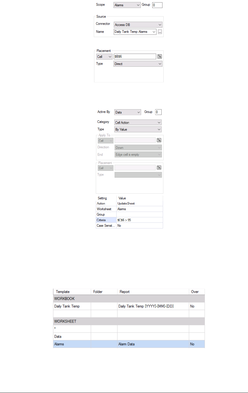
Data Management - 60 -

Another group is configured to retrieve the daily alarms for the tank with the Scope set to the Alarms

worksheet.

For the Data Management, a By Value function is configured.

Active By is set to Data with the Action set to UpdateSheet and the Worksheet set to Alarms. The

Criteria is set for the cell where the daily maximum is written so that the Alarms worksheet is only

updated if that value is > 95.

In order to only show the Alarms report if this criteria is reached, first the Alarms worksheet is hidden

in the template workbook. Then, in Report Names:

The Alarms template worksheet has its Report configured as Alarm Data. This means that if the

Alarms worksheet is updated, it creates the Alarm Data worksheet, makes it visible, and writes the data

to it. Since the Alarms worksheet can only be updated if the criteria is met, this report worksheet is

only generated if the value is > 95.

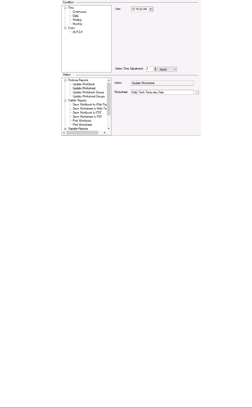
Data Management - 61 -

To generate this report the following action is scheduled:

Notice that only the Data worksheet is scheduled to update.

By Value in Range

The By Value in Range function evaluates the Criteria specified for every value in the Apply To

range and if it is satisfied, triggers the Action specified.

Settings

Action

The Action to trigger if the Criteria is satisfied. This can be UpdateBook, UpdateSheet,

UpdateGroupBook or UpdateGroupSheet.

Worksheet

If the Action is set to UpdateSheet or UpdateGroupSheet, the Worksheet must be set to the name

of a worksheet in the template.

Group

If the Action is set to UpdateGroupBook or UpdateGroupSheet, one or more Group numbers

must be specified. For multiple groups, separate each with a comma.

Criteria

The condition to check and trigger the Action if satisfied. Up to 2 conditions can be specified

each of which can evaluate the value in every cell of the Apply To range.

This is specified by using the Filter Browser (see Filter Range).

Case Sensitive

If the Criteria is text based, set this to Yes to consider case when evaluating.

Example

A daily report template is configured to show hourly averages calculated over the day from a historian.

However, sometimes during the day, the primary historian may go offline and thus the data returned

for that time may be bad (???). However, the system has a secondary historian which does have the

data that is missing. The secondary historian should only be queried if the primary has gone offline

during the day.

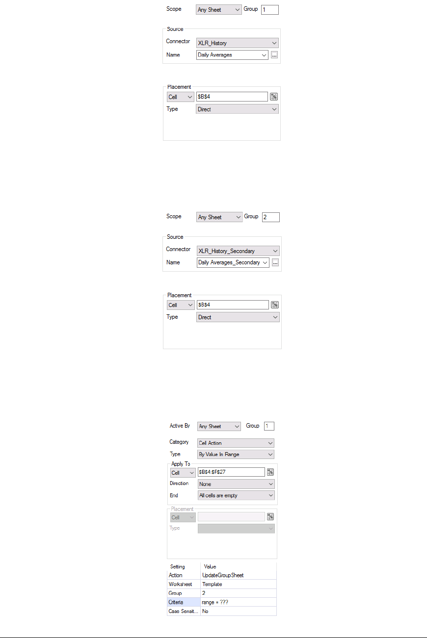
Data Management - 62 -

To accomplish this, first in the project, two connectors must be configured: one to the primary

historian and one to the secondary historian.

In the report template a Data Connection is configured to retrieve the daily data from the primary

historian.

That connection is configured with the Group set to 1.

A second Data Connection is configured to retrieve the daily data from the secondary historian.

That connection is configured with the Group set to 2 with the exact same Placement as the first

connection.

Finally, a Data Management By Value Range function is configured.

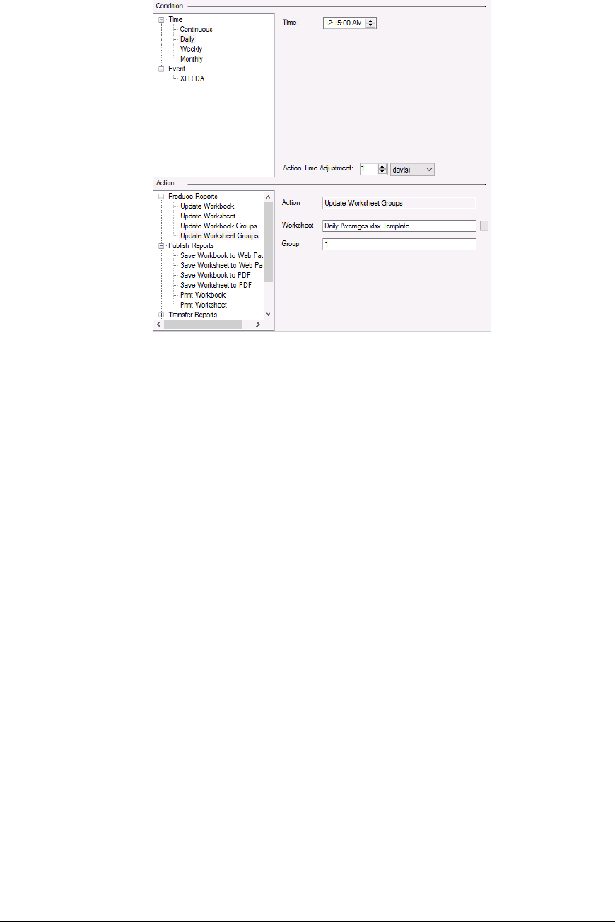
Data Management - 63 -

Notice that this connection is configured for Group 1.

The Criteria is set so if any cell in the range ($B$4:$F$27) is “???”, an UpdateGroupSheet of Group

2 is triggered which retrieves the data from the secondary historian.

To generate this report the following action is scheduled:

Notice that only Group 1 is updated from the Scheduler.

By Row Iteration

The By Row Iteration function goes over each row of the Range specified, setting the cell values in

each row to variables and triggering the Action specified.

The top row of the Range contains the names of the variables to set for each row.

When iterating, if any column in the row contains a formula error, that row is skipped entirely.

Settings

Action

This setting can either be a specific action (selectable from the drop-down list) or a range of cells

each of which contain a fully qualified action to trigger for each row of the Range. For example:

UpdateSheet ‘MyTemplate.xlsx.Template’

PrintSheet ‘MyTemplate.xlsx.Template’ ‘default’

Worksheet

If the Action is set to UpdateSheet or UpdateGroupSheet, the Worksheet field must be set to the

name of a worksheet in the template.

Group

If the Action is set to UpdateGroupBook or UpdateGroupSheet, one or more Group numbers

must be specified. For multiple groups, separate each with a comma.

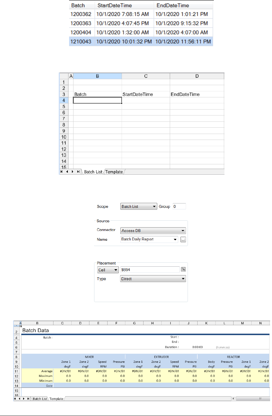
Data Management - 64 -

Example

Consider a report requirement where every day a variable number of batches is produced in a plant and

at the end of the day, a report is required for each batch produced. A table in a database contains a

record for each batch as well as the time it started and ended.

In the template, on the Batch List worksheet the labels are set up for the Batch, StartDateTime, and

EndDateTime.

The database group that returns the batch information over the day is connected to $B$4 in the Batch

List worksheet.

The Template worksheet is set up for the batch report.

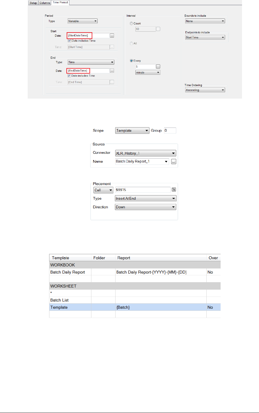
Data Management - 65 -

A history data group is configured for this worksheet to retrieve the data. The Time Period for the

group is set up to use the StartDateTime and EndDateTime returned from the database.

This group is connected to $B$15 on the Template worksheet.

To ensure a workbook is created for every day and contains a report (worksheet) for every batch

produced that day, the Report Names are set as:

For the Template worksheet, the Report is set to use the Batch name returned from the database.

Select Options in the upper right corner and check the box for Hide Template Sheet(s) on report

update.

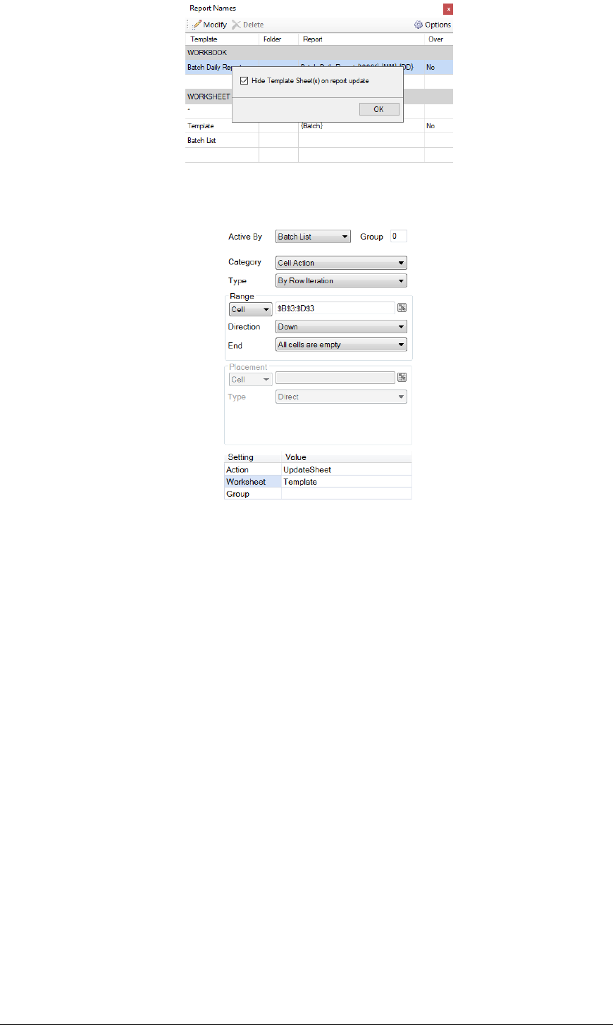
Data Management - 66 -

To trigger a batch report for every record, the By Row Iteration function is configured as:

Notice that Active By is set to Batch List, meaning that this function executes when the Batch List

worksheet is updated.

Also notice that the Range starts at $B$3:$D$3. This is the row containing the headers which are used

as the variables in the template.

Finally, notice that the Action is UpdateSheet to the Template worksheet which means that the

Template worksheet is updated for every row of data returned on the Batch List worksheet starting at

row 4.

To generate the report(s) every day, the following Schedule action should be configured:

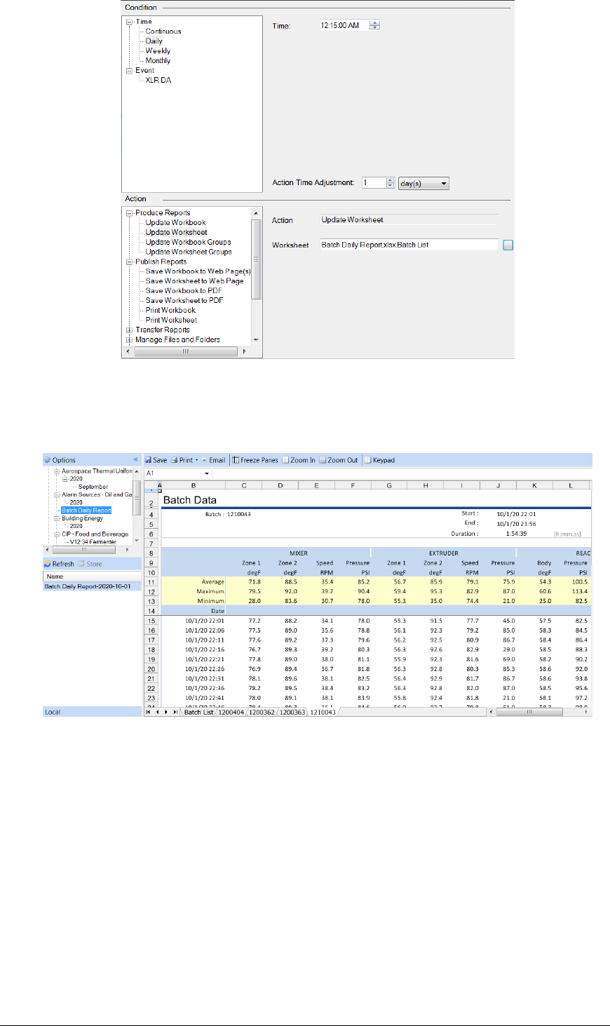
Data Management - 67 -

Note that only the Batch List worksheet is updated from the Scheduler. This in turn will trigger an

update of the Template worksheet for every batch returned from the database.

The net result is a report like this:

Notice that the workbook is named after the day and there is a worksheet for each batch.

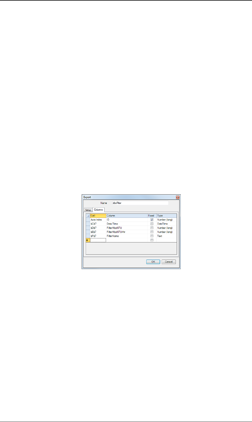
Data Management - 68 -

Data Export

This set of Data Management functions export worksheet data to relational databases (like Microsoft

SQL Server or Access), process tags, XLReporter Functions, or file formats such as CSV and XML.

To Database

The To Database function exports the contents of a cell range to a relational database. The function is

flexible enough to handle the export of either single or multiple rows/columns of data on the worksheet

to single/multiple records in the database.

When data is exported, the values are formatted as they appear in the cells on the worksheet. This

means that the cell(s) should be formatted to adhere to the format required for the column in the

database table being exported to. For example, if a metric requires specific significant figures, the

cells being exported from should be formatted to reflect this.

Settings

Configuration

This is set to the name of a database export file. A browse button is provided to create and

configure these files.

Continue on Fail

Set to Yes to indicate that an export of multiple rows/columns, the export should continue despite

any errors that may occur.

Database Export Builder

The Database Export Builder is used to configure the rules for the export. The settings are stored in a

file with extension asql.

The display contains a Setup tab and either a Columns tab or the Commands tab depending on the

choice made on the Setup tab.

Popup Menus

Popup menus appear when right-clicking rows in the Columns Grid. The following options are

available:

Auto Index

When selected, this indicates that the data exported to the column is determined by the Auto

Index. See the Auto Index section below for more information.

Insert

This inserts a new row in the Columns Grid. A new row can also be inserted by pressing the

Insert button on the keyboard.

Delete

This deletes the row from the Columns Grid. The row can also be deleted by pressing the Delete

button on the keyboard.

Content

Name

This is the name of the configuration.

Data Management - 69 -

Tabs

Setup

Connector

A dropdown list of available connectors which define a connection to a database.

Table

This field indicates the table to use for the export. The dropdown displays a list of all

available tables in the selected Connector. Note that data cannot be exported to a View.

If it is necessary to export to multiple tables, multiple exports must be configured.

Method

Columns

The Columns method is used to link columns from the selected table to cells on the

worksheet. No knowledge of SQL syntax is needed.

Commands

The Commands method is used to execute specific SQL commands on the database

defined in the connector. The SQL syntax must be specified exactly how it is

required by the database.

Bulk Copy

The Bulk Copy method is only available for Connectors to a Microsoft SQL Server

database.

This method exports the entire range of data as defined in the Range settings of the

function to the Table selected, where each column in the range is written to the

corresponding column in the Table.

Columns are exported in the order that the columns are configured in the Table. For

example, if the Table contains the columns: Value1, Value2, Value3 and Value4 and

the Range is $B$4:$E$28, each row of data starting on row 4 are written with values

in B column written to Value1, the C column to Value2 and so on.

If there are less columns in the Range than columns in the Table, the columns that

are not in the Range are set to NULL. If there are more columns in Range than

columns in the Table the Range is truncated to match the number of columns in the

Table.

Data Management - 70 -

Columns

Columns Grid

Cell

This field indicates the cell containing the data to export to the configured column.

Column

This field indicates which column in the database the data will be exported to.

Fixed

This indicates that the cell reference will remain fixed in place even if the

management connection has been configured to export a dynamic range.

For example, a database table has 5 columns including a Timestamp column and 4

data columns, and a daily report has a timestamp in cell $A$1 and 4 columns

containing the day’s data within the cell range of $B$4:$E$27. We can configure

our data export to use the timestamp in $A$1 for each record in the cell range by

assigning the cell to the Timestamp column and checking Fixed.

Type

This field displays the data type of the selected column in the database. See the

Database Management section of this document for more information on data

types.

Note that when the data type of a column is modified in the database, the export

group needs to be re-configured. From the Setup tab, change the Export Table

section and then re-select the Table.

Commands

In the grid, specify SQL commands (some level of SQL is required). A command

can contain a cell reference enclosed in curly brackets e.g., {$A$1}. When a cell

reference uses the $ symbol, it remains fixed while the range is exported. If the $ is

not used, the value changes for every row/column in the Source range.

Auto Index

When exporting to more than one table, an Auto Index can be used to maintain a relationship between

the tables. The Auto Index is a number that is incremented after the completion of an UpdateSheet or

UpdateBook action so while the action is in progress, each export will use the same index value.

For example, suppose a database contains two tables. One table contains the columns Batch ID,

BatchStartTime and BatchEndTime, and the other table contains the process data for each batch. If an

Auto Index is used a unique relationship can be made between the tables during the export operation.

Creating the Auto Index Table

The Auto Index table can be created using the Database Manager application. Connect to the

database where the data will be exported.

Select Add to create a new table. Set Name to AutoIndex. Under Columns in the first row, set Name

to ID and Type to Number (long). Click OK to create the table.

Usage

To use the Auto Index feature each database table that will be used must contain a column for the

Index, and the data type must be Number (Long). When configuring the Cell for the Column, right

click and select Auto Index. Note that when exporting to tables in two separate databases, the

AutoIndex is determined by the table in the first export.

Example

A daily report is required showing hourly maximums over the day for tanks and extruders. In addition,

the daily maximum for each tank and extruder is displayed using MAX functions within the worksheet.

A second, monthly report is required to display the daily maximums for the month.

While it is possible to get the daily maximums for the month from the historian, this requires a lot of

number crunching on the historian. Since the daily report already has these values it would be less

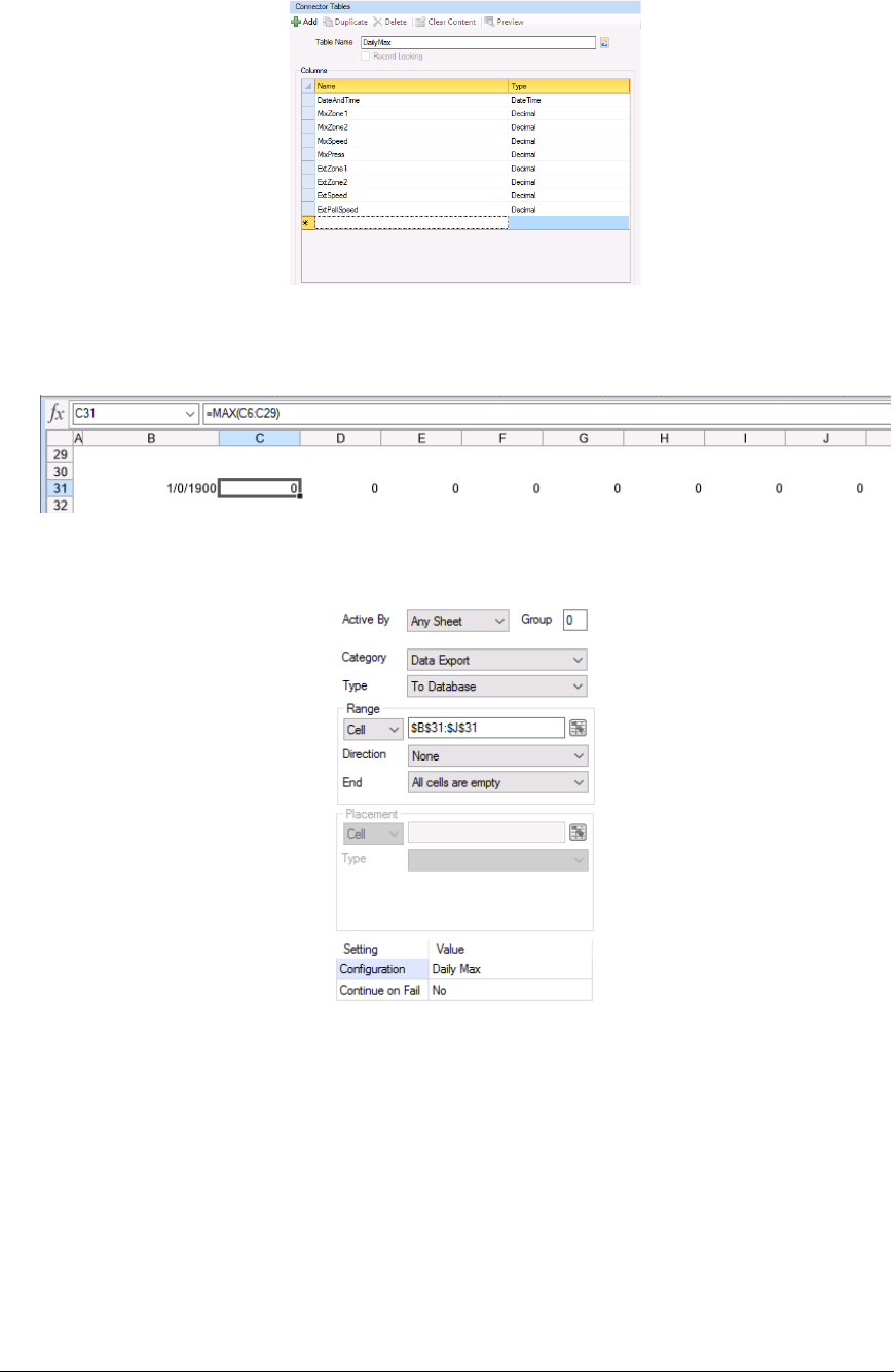
Data Management - 71 -

taxing to log the daily maximums to a database and then retrieve these values from the database for the

monthly report.

The first thing to configure is a database table to hold the daily maximums. XLReporter provides the

Database Manager application to perform this function.

The daily report template is set up with the daily maximum calculations beneath where the hourly

maximums for the day are placed.

To export the daily maximums to the database a Data Export To Database function is configured:

Notice the Range is set to $B$31:$J$31 with Direction set to None so that only row 31 is exported.

In the Configuration itself:

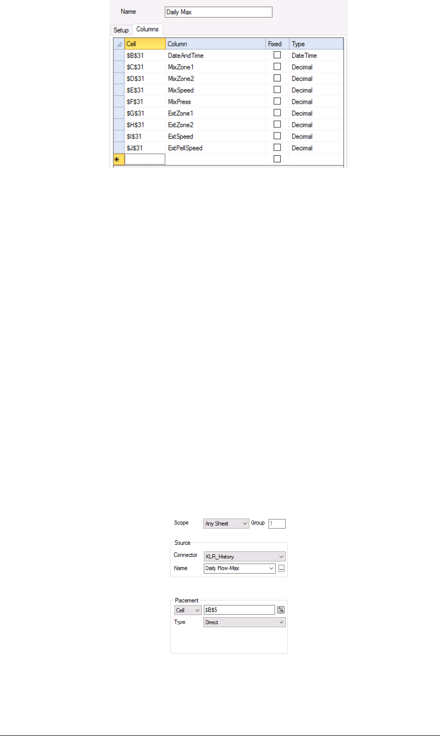
Data Management - 72 -

Each Column is configured with the corresponding cell in row 31.

Now in the monthly report template a data group can be configured to retrieve the data from this

database table.

To Variables

The To Variables function exports the contents of cells(s) to XLReporter variables. The variables

can either be Function variables defined in the project (like a Register), Memory variables or Custom

variables. Variables can be selected from the browser or manually entered at the top of the browser.

Settings

Input Cell (up to 4)

The cell containing the value to export to variable.

Variable (up to 4)

The variable to export the cell value to.

Example

A daily report is required to retrieve the maximum flow rate over the day and the time that it occurred.

Then, a set of process values need to be retrieved at the time the maximum flow rate occurred for

analysis purposes.

To accomplish this, first a Data Connection is configured to retrieve the daily maximum and the time

that it occurred.

Notice this connection is configured for Group 1.

A second data connection is configured to retrieve the sample values at the time that maximum

occurred.

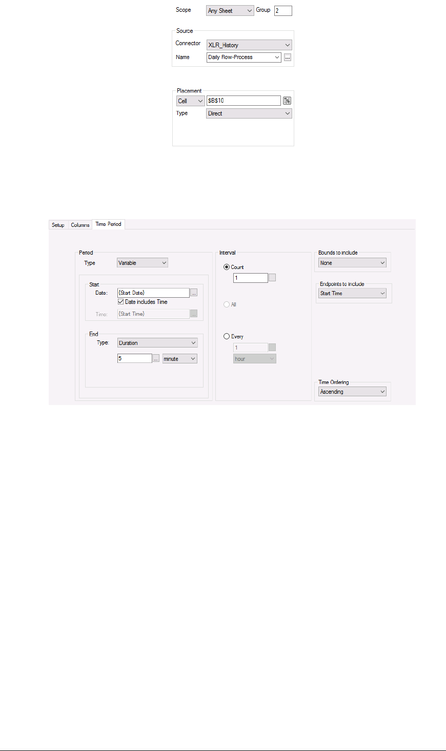
Data Management - 73 -

Notice this connection is configured for Group 2.

Looking at the group itself, under the Time Period tab,

The Type is set to Variable with the Start Date set to {Start Date}. This variable needs to be set with

the time of the maximum flow rate for the day.

To set this, a Data Management To Variable function is configured.

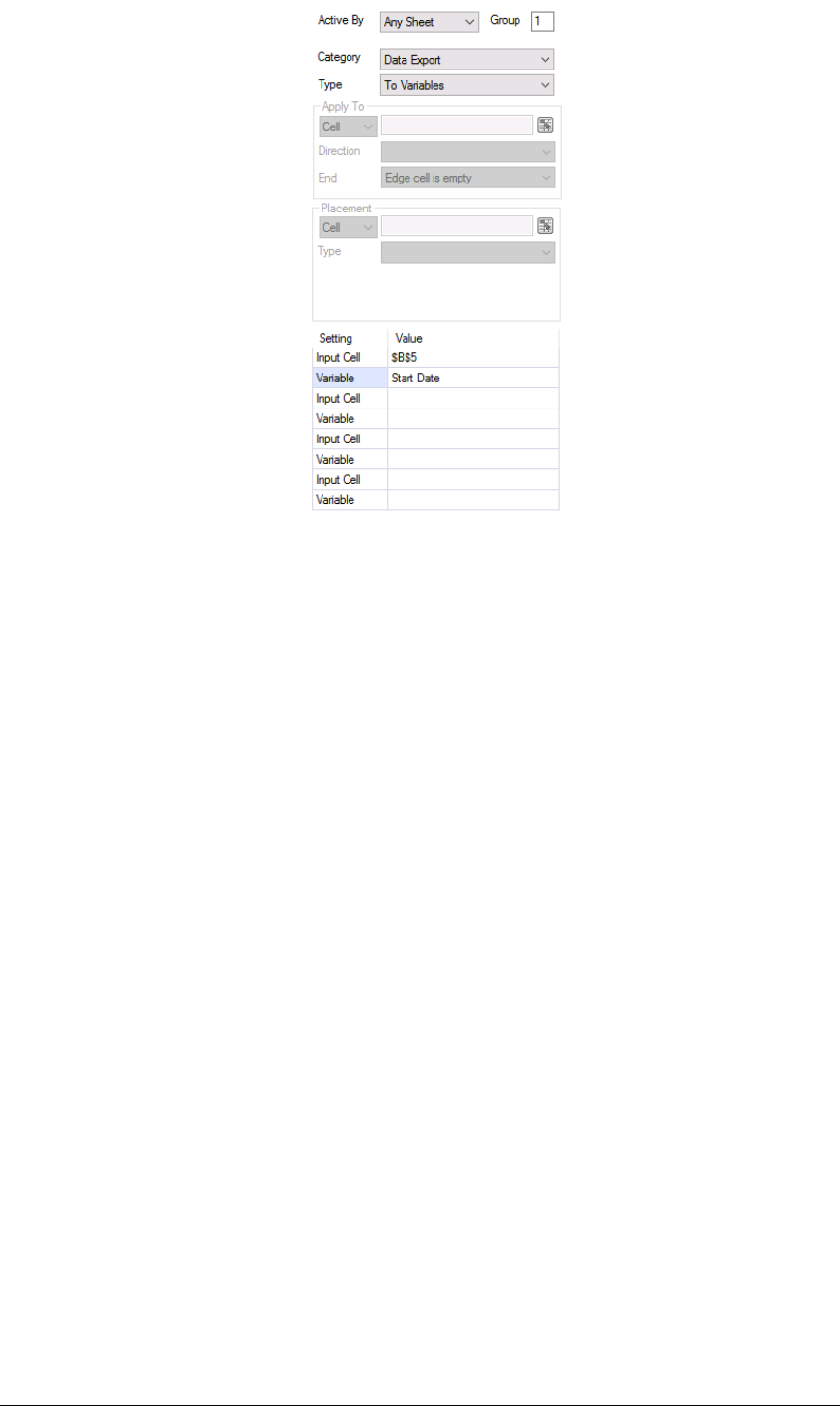
Data Management - 74 -

The Start Date Variable is set to Cell $B$5 which contains the time the maximum flow rate occurred.

This connection is also set to Group 1 so that the variable is set before the process data is retrieved.

In the Scheduler there are 2 actions required to run: the update of group 1 and then the update of group

2. These can be scheduled to run at same time as long as the group 1 update is listed first.

To Variable List

The To Variable List function exports the contents of cells to XLReporter Variables based on a

Configuration specified. This is an alternative to the To Variables function if more than 4 values

need to be exported.

Settings

Configuration

The configuration that defines the variables and cells containing the data to export. The Variable

Export Builder is used to perform this (see below).

Variable Export Builder

The Variable Export Builder builds the configuration file that is used to export data from cells to

variables in the project. The settings are stored in a file with extension avxp.

Under the Variable List tab specify the Cell and Variable name for every variable that should be

exported to. Note that Function, Memory and Custom variables are all supported. A browser is

provided to select the variable, or it can be manually entered at the top.

Example

A factory generates a report on ten machines every time a machine cycle ends. The report for each

machine is identical except for the source tags. Instead of setting up ten different report templates, a

single template can use variables for the tag names.

A history group is used as the data source and would be configured with variables as follows:

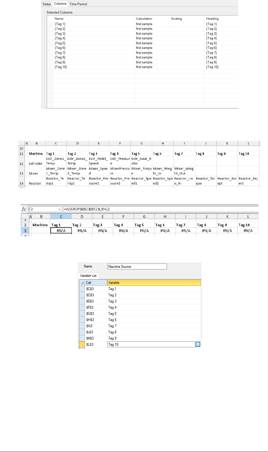
Data Management - 75 -

A second template is configured to provide the values for the variables using a lookup table with a row

for each of the ten machines and a column for the corresponding source tags for that machine as

follows:

The worksheet also contains VLOOKUP in row 3 which select the tags based on the Machine name is

B3. For example, if B3 is set to Reactor then the C3:L3 will contain the reactor tag names.

The tags in row 3 are passed to the variables used by the history group using a

To Variable List management function.

Whenever a machine cycle ends, the variable for the machine name is set, this lookup template is

updated to set the source tag variables and then the report template is updated to generate the report for

the machine.

To Tag List

The To Tag List function exports the contents of many cells to (real time) process tags based on a

Configuration specified.

Before exporting, the formatting of the cells that contain the source data is changed to the format of the

named cell Format_Normal. If the named cell does not exist, the background color of the source data

is cleared.

Data Management - 76 -

In the event that either the writing or reading (if Readback set to Yes) fails, the cell formatting is

changed according to the following:

a) Write Fail: the cell formatting is modified to the format of the named cell Format_WriteFail. If

the named cell does not exist, the background color of the source data is set yellow.

b) Read Fail: the cell formatting is modified to the format of the named cell called

Format_ReadFail. If the named cell does not exist, the background color of the source data is set

red.

In the event that the writing and reading (if Readback set to Yes) is successful, the cell formatting is

changed to the format of the named cell Format_Success. If the named cell does not exist, the

background color is unchanged.

Note that the formatting of the named cell Format_Success will overwrite any existing formatting in

the source data.

Settings

Configuration

The configuration that defines the process tags and cells containing the data to export. The Tag

Export Builder is used to perform this (see below).

Readback

If set to Yes, after the cell values are written to the process tags a readback is performed to verify

the values have been written correctly.

Wait Time

If Readback is set to Yes, the amount of time (in seconds) to wait between writing the values and

performing the readback.

Readback Tolerance

If Readback is set to Yes the tolerance where if the value read back compared to the value written

is within the tolerance, the write is considered a success.

Fail Count

To display a count of how many tags failed to export or readback, set this to a cell reference,

otherwise it can be left blank.

Tag Export Builder

The Tag Export Builder builds the configuration file that is used to export data from cells to tags in the

real time server. The settings are stored in a file with extension atxp.

Under the Setup tab specify the Connector to the real time database to export data to.

Under the Tag List tab specify the Cell, Tag and Tag Type for every tag data should be exported to.

If there is an array of tags to export data to, they can be specified as a single entity. The configuration

is identical to that of a single tag connection and can contain

[start direction end] where,

start start index

direction the direction the values will be read from the worksheet

end end index

For example, suppose $A$4 is assigned to Temperature[01-12]. The values from $A$4 to $L$4 will be

exported to Temperature01 to Temperature12.

Suppose $A$4 is assigned to Temperature[01|12]. The values from $A$4 to $A$15 will be exported to

Temperature01 to Temperature12.

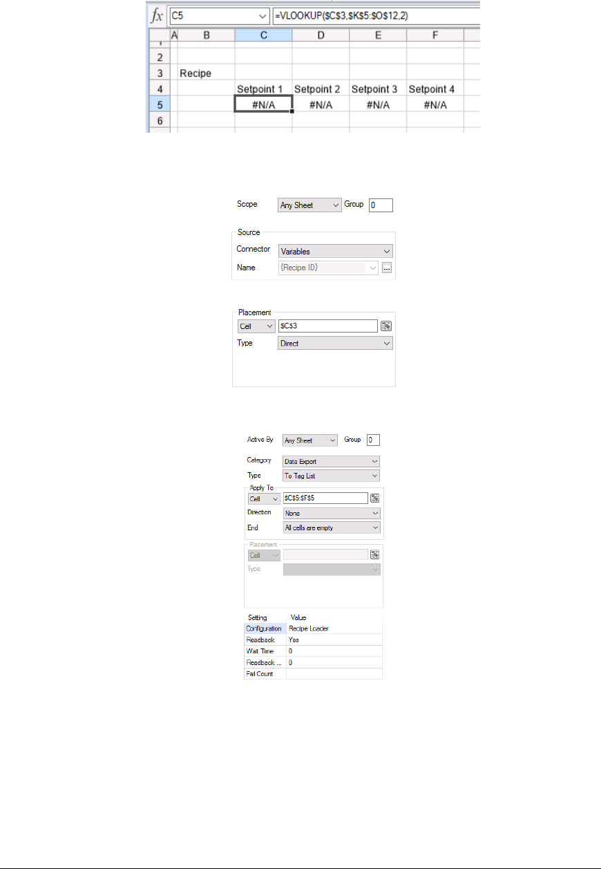
Data Management - 77 -

Example

A report template is configured with a list of recipe IDs along with four set points for the recipe that

must be downloaded to the PLC before the recipe can be produced. The recipe table in in cells

$K$5:$O$12.

In the worksheet VLOOKUP functions are used to get the four set points based on the recipe ID

specified.

The recipe is entered by setting a variable. The variable is set as a Data Connection in the template.

To download the set points to the PLC a Data Export To Tag List function is configured.

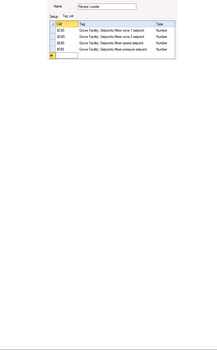
Data Management - 78 -

In the Configuration itself,

Each set point is set to the corresponding cell on the worksheet.

There are multiple ways that the variable for the Recipe ID can be set including from a value in the

PLC or from a prompt in an On Demand report. The key is that when the report is updated, the Recipe

is written in which causes the formulas to update with the set points which then get downloaded to the

PLC.

Range to Text

The Range to Text function exports a range of cells to a text file in the file format specified.

Settings

Format

The file format for the text file can be CSV (Comma Delimited) or Text (Tab Delimited) format.

Directory

The directory where the text file is stored. If this is left blank, the text file is stored in the Reports

Directory of the current project (as defined in the Project Explorer). If this is not a full path

reference, the setting is used as subfolders of the Reports Directory. If any part of the directory

does not exist, it is created.

This setting may also be specified as a cell reference where the cell reference contains the

directory.

File

The name of the text file to export the range to with or without a file extension. If the file

extension is not specified derived from the Format setting (either CSV or TXT).

If this setting is left blank, the text file is named after the target workbook and worksheet (as

specified in the template) in the format Workbook_Worksheet.FileExtension where FileExtension

is either CSV or TXT depending on the Format setting.

Note that keywords for the date and time can be entered for the file name e.g., entering

{MMM}_{DD}_{YYYY}.csv will name a report generated on June 1

2020 Jun_1_2020.csv. See

the Name Types chapter for the full list of supported keywords. Note that some keywords, such

as {DATIM} contain illegal file name characters when evaluated. These keywords cannot be used

for the file name.

This setting may also be specified as a cell reference.

Overwrite

If set to Yes, the text file is overwritten if it exists. If set to No and the file exists, nothing is done.

Data Management - 79 -

Example

A report template is designed to show 15 minute samples as well as daily summaries and a chart of the

samples throughout the day. Those 15 minute samples need to be exported to a csv file so that can be

imported into a data analysis system which keeps track of the entire facility.

To export the 15 minute samples a Range to Text function is used. If the data range starts at

$B$8:$H$8, the settings are:

Range $B$8:$H$8, Down, All cells are empty

Setting

Format CSV (Comma Delimited)

Directory \\FileServer\Analysis

File {YYYY}-{MM}-{DD}.csv

Overwrite No

Where FileServer is the name or IP address of the target location.

Worksheet to Text

The Worksheet to Text function exports an entire worksheet in the workbook to a text file in the file

format specified.

Setting

Format

The file format for the export file in either CSV or Text formats.

Directory

The directory where the text file is stored. If this is left blank, the text file is stored in the Reports

Directory of the current project (as defined in the Project Explorer). If this is not a full path

reference, the setting is used as subfolders of the Reports directory. If any part of the directory

does not exist, it is created.

This setting may also be specified as a cell reference where the cell reference contains the

directory.

File

The name of the text file with or without a file extension. If the file extension is not specified then

it is either CSV or TXT according to the Format setting.

If this setting is left blank, the text file is named after the target workbook and worksheet (as

specified in the template) in the format Workbook_Worksheet.FileExtension where FileExtension

is either CSV or TXT.

Note that keywords for the date and time can be entered for the file name e.g., entering

{MMM}_{DD}_{YYYY}.csv will name a file generated on June 1

2020 Jun_1_2020.csv. See the

Name Types chapter for the full list of supported keywords. Note that some keywords, such as

{DATIM} contain illegal file name characters when evaluated. These keywords cannot be used for

the file name.

This setting may also be specified as a cell reference.

Overwrite

If set to Yes, the text file is overwritten if it exists. If set to No and the file exists, nothing is done.

Data Management - 80 -

Example

An analysis application requires 15 minute samples on equipment over the day to monitor how

efficiently the plant is operating. That application cannot directly interface with the process historian

but can import CSV files.

In this case, XLReporter can act as middleware to get the data from the process historian and export

the CSV file for the analysis application. To accomplish this, a history data group is configured to

retrieve the 15 minute samples and a Worksheet to Text management function is configured to export

the data to CSV. The settings are:

Setting

Format CSV (Comma Delimited)

Directory \\FileServer\Analysis

File {YYYY}-{MM}-{DD}.csv

Overwrite No

Where FileServer is the name or IP address of the target location.

Range to XML (Schema)

The Range to XML (Schema) function saves an XML file based on the range specified by using an

XML Schema defined by the user.

Before this function can be used, an XML Schema needs to be created. To create an XML Schema,

copy the sample schema file below and paste it in Notepad. Save this file with the extension XSD.

An element name is needed for each column that is exported. The syntax for element name is

<xsd:element name="Time" type="xsd:time"/>. The text “Time” is the column heading and the text

“xsd:time” is referring to the data type. Add an element name sequence for each column that is

exported and remove any extra element name sequences.

Sample Schema

<?xml version="1.0" encoding="UTF-8" standalone="no" ?>

<xsd:schema xmlns:xsd="http://www.w3.org/2001/XMLSchema">

<xsd:element name="Schema">

<xsd:complexType>

<xsd:sequence>

<xsd:element minOccurs="0" maxOccurs="unbounded" name="Data">

<xsd:complexType>

<xsd:sequence>

<xsd:element name="Time" type="xsd:time"/>

<xsd:element name="Operator" type="xsd:string"/>

<xsd:element name="Flow" type="xsd:int" />

</xsd:sequence>

</xsd:complexType>

</xsd:element>

</xsd:sequence>

</xsd:complexType>

</xsd:element>

</xsd:schema>

Settings

Schema

The name of the XML Schema used to perform the export to the XML file. If this is entered

without a fully qualified path e.g., C:\XLRproject\Data\mySchema, the schema file must be

located in the Data folder of the project.

Data Management - 81 -

Directory

The directory where the XML file is stored. If this is left blank, the text file is stored in the

Reports Directory of the current project (as defined in the Project Explorer). If this is not a full

path reference, the setting is used as subfolders of the Reports Directory. If any part of the

directory does not exist, it is created.

This setting may also be specified as a cell reference.

File

The name of the XML file to save. If this is left blank, the file is named after the target workbook

and worksheet (as specified in the template) in the format Workbook_Worksheet.xml.

Note that keywords for the date and time can be entered for the file name e.g., entering

{MMM}_{DD}_{YYYY} will name a file generated on June 1

2020 Jun_1_2020.xml. See the

Name Types chapter for the full list of supported keywords. Note that some keywords, such as

{DATIM} contain illegal file name characters when evaluated. These keywords cannot be used for

the file name.

This setting may also be specified as a cell reference.

Table

The XML table in the schema file to use. If this field is left blank, the first table in the schema file

will be used.

Mode

Overwrite

If the XML file exists it is overwritten with the latest data.

Append

The latest data is appended to the XML file once it exists.

Example

An analysis application requires 15 minute samples on equipment over the day to monitor how

efficiently the plant is operating. That application cannot directly interface with the process historian

but can import XML files and provides a schema for the XML structure.

In this case, XLReporter can act as middleware to get the data from the process historian and export

the XML file for the analysis application. To accomplish this, a history data group is configured to

retrieve the 15 minute samples and a Range to XML management function is configured to export the

data to XML.

If the data starts in $B$8:$H$8, the settings are:

Range $B$8:$H$8, Down, All cells are empty

Setting

Schema C:\Analysis\schema.xsd

Directory \\FileServer\Analysis

File {YYYY}-{MM}-{DD}.xml

Table Data

Mode Append

Where FileServer is the name or IP address of the target location.

Data Management - 82 -

Sheet to Workbook

The Sheet to Workbook function is used to export the current worksheet from the report to another

Excel workbook.

Settings

Directory

The directory where the Excel workbook to export the worksheet to exists. If this is left blank, the

Reports Directory of the current project is used (as defined in the Project Explorer). If this is

not a full path reference, the setting is used as subfolders of the Reports Directory.

This can be a fixed name or cell reference and can contain XLReporter Name Types like

{YYYY}, {MMM}, etc.

Workbook Name

The name of the workbook to export the worksheet to.

This can be a fixed name or cell reference and can contain XLReporter Name Types like

{YYYY}, {MMM}, etc.

If this setting contains a full path, that path is used as the Directory.

If the Workbook does not exist, it will be created.

Target Sheet

If this setting is specified, when the worksheet is copied to the workbook it is renamed to what is

specified, otherwise the name of the worksheet in the report is used.

Overwrite

If Overwrite is set to Yes and the Target Worksheet name exists in the Target Workbook, it is

deleted and the new worksheet from the source is inserted as the last worksheet tab in the Target

Workbook.

If Overwrite is set to No and the worksheet name already exists in the workbook being exported

to, the following occurs:

• If the Target Sheet is specified, nothing is exported.

• If the Target Sheet is not specified, the sheet is renamed as Target Book-Target Sheet in

the target workbook.

Example

A batch report template is created to show all the data collected over a specific batch. This template

contains one worksheet, and each batch report is its own workbook. However, management would like

to be able to compare all the batches run over the day by having a workbook for the day that has a

worksheet for every batch run.

To accomplish this, a Sheet to Workbook management function is configured in the batch report

template to copy the batch report worksheet to the daily report workbook for management. The

settings are:

Setting

Directory Daily Batch

Workbook Name Daily Batch {YYYY}-{MM}-{DD}

Target Sheet {RG000}

Overwrite No

Note, RG000 holds the name of the batch.

Data Management - 83 -

Range to Workbook

The Range to Workbook function is used to export a range of cells from the report to a worksheet in

another Excel workbook.

Settings

Directory

The directory where the Excel workbook to export the range to exists. If this is left blank, the

Reports Directory of the current project is used (as defined in the Project Explorer). If this is

not a full path reference, the setting is used as subfolders of the Reports Directory.

This can be a fixed name or cell reference and can contain XLReporter Name Types like

{YYYY}, {MMM}, etc.

Workbook Name

The name of the workbook to export the range to. The workbook must exist, it will not be created.

This can be a fixed name or cell reference and can contain XLReporter Name Types like

{YYYY}, {MMM}, etc.

If this setting contains a full path, that path is used as the Directory.

Target Sheet

The worksheet in the workbook to export the range to.

Target Cell

The cell in the Target Sheet to paste the exported range to. This cell is the upper left-hand corner

of where the data should be pasted.

Note, if merged cells are to be exported, the Target Cell should encompass the entire range of the

merge. For example, if you are exporting cell $B$4 to cell $D$7 and $B$4 is merged from B4 to

D4, then the Target Cell should be $D$7:$F$7.

Paste

This setting defines what to paste from the range to the Target Cell. If the range to export

contains formulas to other worksheets it is recommended to use the Values or Values and Formats

setting, otherwise the formulas may result in errors in the exported workbook.

Example

A daily report template is created to show all the data collected over the day as well as a summary of

information collected. However, management has a workbook they manually create every month with

sheets for every day which requires the daily summary data from these reports.

Rather than have them copy and paste manually from the daily reports, a Range to Workbook

management function is configured in the daily report template to copy the summary information from

the worksheet to the monthly workbook.

If the summary data is in cells $B$4:$H$8, the settings are:

Range $B$4:$H$8, None, All cells are empty

Setting

Directory \\FileServer\Monthly Operations

Workbook Name Monthly Operations {MMM}-{YYYY}

Target Sheet {DD}

Target Cell $B$4

Paste Values

Where FileServer is the name or IP address of the target location.

Data Management - 84 -

Data Import

This set of Data Management functions import data from workbooks, worksheets, text files, xml files,

and Excel Add-ins.

Range From Workbook

The Range From Workbook function is used to import data from an outside workbook to a

Placement Cell location in the current workbook.

Settings

Directory

The directory where the Excel workbook to import the range from exists. If this is left blank, the

Reports Directory of the current project is used (as defined in the Project Explorer). If this is

not a full path reference, the setting is used as subfolders of the Reports Directory.

This can be a fixed name or cell reference and can contain XLReporter Name Types like

{YYYY}, {MMM}, etc.

Workbook Name

The name of the workbook to import the range from.

This can be a fixed name or cell reference and can contain XLReporter Name Types like

{YYYY}, {MMM}, etc.

If this setting contains a full path, that path is used as the Directory.

In addition, the Workbook Name can be specified with a wildcard. This changes the setting from

a specific file name to a filter that is used to get the most recent file in the Directory specified.

For example, a Workbook Name of Flow*.xlsx would import data from the most recent file in the

Directory that starts with Flow and ends with .xlsx.

Start

If Start is intended to be a reference to a range found on the worksheet, it must be set as a single

cell and the value in the cell must be a cell range containing “$”, e.g., “$B$30:$D$30”.

Otherwise, this can be set to the entire range to import.

Direction

This setting defines the Direction in which to expand the Start by in order to determine the entire

range of data to import.

Until

This setting defines how to terminate the detection of the range to import.

Paste

This setting defines what to paste from the range to the Placement. If the range to import contains

formulas to other worksheets it is recommended to use the Values or Values and Formats setting,

otherwise the formulas may result in errors in the report workbook.

Example

To extract summary data existing in a June monthly worksheet in a workbook called

MyReport2020.xlsx the following settings would be used:

Data Management - 85 -

Placement

Cell $B$4

Type Offset

Direction Down

Offset dM

Setting

Directory C:\Reports

Workbook Name MyReport{YYYY}

Worksheet {MMMM}

Start $B$30:$D$30

Direction None

Until All cells are empty

Paste All

Range From Workbook List

The Range From Workbook List function has the same functionality as the Range From Workbook

function but operates on a list of parameters specified as a table in a worksheet in the template. This

allows multiple ranges from multiple worksheets to be imported using a single action.

Sheet From Workbook

The Sheet From Workbook function is used to import an entire Source Sheet to a Target Sheet.

Settings

Directory

The directory where the Excel workbook to import the worksheet from exists. If this is left blank,

the Reports Directory of the current project is used (as defined in the Project Explorer). If this

is not a full path reference, the setting is used as subfolders of the Reports Directory.

This can be a fixed name or cell reference and can contain XLReporter Name Types like

{YYYY}, {MMM}, etc.

Workbook Name

The name of the workbook to import the worksheet from.

This can be a fixed name or cell reference and can contain XLReporter Name Types like

{YYYY}, {MMM}, etc.

If this setting contains a full path, that path is used as the Directory.

In addition, the Workbook Name can be specified with a wildcard. This changes the setting from

a specific file name to a filter that is used to get the most recent file in the Directory specified.

For example, a Workbook Name of Flow*.xlsx would import data from the most recent file in the

Directory that starts with Flow and ends with .xlsx.

Source Sheet

The name of the worksheet to import.

Target Sheet

If specified, when the worksheet is imported into the report workbook this name is applied.

Otherwise, the worksheet name is not changed.

If the target sheet name already exists in the report workbook, the name is rebuilt as Workbook

Name-Target Sheet (truncated to 31 characters). If that sheet exists, a default name (e.g., Target

Sheet (2)) is used.

Data Management - 86 -

Hyperlink Cell

A hyperlink can be added to the sheet(s) imported to navigate back to the Active By worksheet

which may contain summary information about the worksheet(s) imported. Hyperlink Cell

determines which cell the hyperlink will appear in on the imported sheet(s).

Hyperlink Text

This is the text that will appear in the cell for users to click on. If the cell is specified and the text

is not, the Active By sheet name will appear as the text.

Overwrite

If Overwrite is set to Yes and the Target Worksheet name exists in the workbook, it is deleted

and the new worksheet is inserted as the last worksheet tab in the Target Workbook.

If Overwrite is set to No and the worksheet name already exists in the workbook the name is

reconfigured as Workbook Name-Target Sheet. If a sheet with that name exists, the worksheet is

named Target Sheet (x) where x is a number starting at 2.

Example

To move an entire monthly June worksheet from workbook named Station_1_2020 and rename the

June worksheet to ST_1 in a summary workbook the following settings would be used:

Setting

Directory C:\Reports

Workbook Name Station_1_{YYYY}

Source Sheet {MMMM}

Target Sheet ST_1

Hyperlink Cell

Hyperlink Text

Overwrite No

Sheet From Workbook List

The Sheet From Workbook List function has the same functionality as the Sheet From Workbook

function but operates on a list of parameters specified as a table in a worksheet in the template. This

allows multiple ranges from multiple worksheets to be imported using a single action.

From Text File

The From Text File function imports the content of a text file into a worksheet.

Settings

Directory

The directory where the text file to import exists. If this is left blank, the Reports Directory of

the current project is used (as defined in the Project Explorer). If this is not a full path reference,

the setting is used as subfolders of the Reports Directory.

This can be a fixed name or cell reference and can contain XLReporter Name Types like

{YYYY}, {MMM}, etc.

Text File

The name of the text file to import.

This can be a fixed name or cell reference and can contain XLReporter Name Types like

{YYYY}, {MMM}, etc.

If this setting contains a full path, that path is used as the Directory.

Data Management - 87 -

In addition, the Text File can be specified with a wildcard. This changes the setting from a

specific file name to a filter that is used to get the most recent file in the Directory specified. For

example, a Text File of Flow*.csv would import data from the most recent file in the Directory

that starts with Flow and ends with .csv.

Delimiter

This setting defines how the values are separated in the file. A drop-down list of common

separators is provided to select from or a custom delimiter can be manually entered.

Rows in Header

This setting defines how many rows in the text files should be considered header rows. If the

Placement Type is set to any of the Insert options, when the text file data is written, the header

rows will appear at the top/left base on the Placement Cell and Direction without any inserting,

and then the data itself is inserted. For any other Placement Type this setting is ignored.

Example

To extract the content of an hourly CSV file directly into an Excel workbook the following settings

would be used:

Placement

Cell $B$4

Type Offset

Direction Down

Offset hD

Setting

Directory C:\MyCSVFiles

Text File {YY}{MM}{DD}_{hh}_Station 1.CSV

Delimiter Comma

Rows In Header 0

From XML File

The From XML File function is used to import data from a specific Table in an XML file.

Settings

Directory

The directory where the XML file to import from exists. If this is left blank, the Reports

Directory of the current project is used (as defined in the Project Explorer). If this is not a full

path reference, the setting is used as subfolders of the Reports Directory.

This can be a fixed name or cell reference and can contain XLReporter Name Types like

{YYYY}, {MMM}, etc.

XML File

The name of the XML file to import.

This can be a fixed name or cell reference and can contain XLReporter Name Types like

{YYYY}, {MMM}, etc.

If this setting contains a full path, that path is used as the Directory.

In addition, the XML File can be specified with a wildcard. This changes the setting from a

specific file name to a filter that is used to get the most recent file in the Directory specified. For

example, an XML File of Flow*.xml would import data from the most recent file in the Directory

that starts with Flow and ends with .xml.

Data Management - 88 -

Table

This setting is the name of the table in the XML file to import data from. If there are multiple

tables in the file to import data from, each must be specified in their own Management connection.

Headings

This setting determines how the column headings in the Table are handled.

• None

This indicates that only data is imported into the report from the file. Every column is

imported in the order it is shown in the file.

• From File

This indicates that the column headings of the table in the file are shown as the top row with

the data in subsequent rows beneath. Every column is imported in the order it is shown in the

file.

• From Sheet

This indicates that the headings are from the worksheet, one row above the Placement Cell

specified. The headings from the sheet determine which headings are imported from the table

in the file as well as the order in which they are displayed in the report. With the setting, the

headings from the sheet must match exactly with the column names in the table in the file.

For example, if the table in the file consists of the columns Flow, Speed, Pressure, Temp and

Timestamp but you only want to show Timestamp and Speed data starting in $B$4, in $B$3

enter Timestamp and in $C$3 enter Speed.

Example

A third-party software vendor produces an XML file every day containing data that needs to be

brought into a daily report alongside process data that XLReporter can access directly.

To bring in the data from the XML file a From XML File function is configured. The settings are:

Placement

Cell $B$4

Type Direct

Setting

Directory C:\MyXMLFiles

XML File {YY}{MM}{DD}.xml

Table Data

Headings None

From Add-in Formulas

The From Add-in Formulas function is used to import data from formulas provided by 3

party add-

ins in Excel. This allows reports to be more “portable” as now the data from these add-in formulas can

be viewed by anyone as there is no more add-in dependency.

Settings

Add-in

If the Add-in providing the formulas is an xla or xlam file, specify the name of it for this setting.

Remove Formulas

Typically, the add-in formulas should be removed in the final report. To do so, set this to either

All or Range. All removes every formula on the report worksheet while Range removes the

formulas specifically from the Range specified.

Range

If Remove Formulas is set to Range, the cell reference specified for this setting will have all

formulas removed so that just the values remain.

Data Management - 89 -

Alternatively, this can be set to the start of an array formula reference anywhere in the workbook.

When set to this, any range of cells containing this formula reference is removed leaving only the

values behind. Additionally, if the Add-in specified is for the PI DataLink from OSIsoft

(Pidldialogs), any range of array formulas is triggered to resize before the formulas are removed.

In order for this to work the PIdldialogs add-in must installed in Excel. To install, in Excel select

File, Options. In Excel Options select Add-ins on the left.

On the right, click the Go button for Manage. If PidlDialogs is listed, make sure it is checked. If

it is not listed, click the Browse button to add it.

If the PI server has been installed by a third-party like Rockwell Software or Emerson Automation

Solutions browse to the installation folder for the historian of that software and then to PIPC\Excel

and select pidldialogs.xla.

If the PI server has been installed directly from OSIsoft, locate the folder where PI DataLink is

installed, browse to the Excel folder beneath it and select pidialogs.xla.

Make sure PIdldialogs is checked and click OK to install.

Note, in order for this function to work, a licensed copy of Microsoft Excel must be installed on the

system.

Example

A report template is configured with multiple sets of formulas from the PI DataLink add-in across

multiple worksheets. All the formulas use timestamps written to cells $A$1 and $A$2 which are

configured as Variable connections in the template. The time duration varies and the formulas must be

removed so that the report can be viewed on systems where the PI DataLink add-in is not installed.

To accomplish this, a From Add-in Formulas function is configured. The settings are:

Setting

Add-in Pidldialogs

Remove Formulas Range

Range =PI

With these settings, every range containing an array formula starting with =PI is refreshed and then the

formulas removed leaving just the values behind.

Function

The following management functions simplify some of the functionality that could be done by using

workbook functions and formulas.

Delete Worksheet

The Delete Worksheet function deletes the specified worksheet from the report. This is useful if the

worksheet is being used for “temporary” calculations for the final report workbook. Before applying

this function, make sure that that there are no links referencing it from other sheets.

Settings

Worksheet

The name of the worksheet to delete. This can be a fixed name or a cell reference where the cell

contains the name of the worksheet to delete.

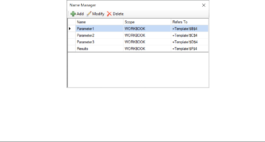
Data Management - 90 -

Active Worksheet

The name of the worksheet to activate after the Worksheet specified is deleted. This can be

blank, a fixed name or a cell reference where the cell contains the name of the worksheet to

activate.

If left blank and the worksheet to delete is the active worksheet, the next worksheet to the right

becomes active. If the worksheet is the rightmost worksheet, then the worksheet immediately to

the left becomes active.

Range

The range to select on the Active Worksheet if it is specified. This can be left blank if it is not

needed.

Example

An On Demand batch report is used to compare multiple batches. This report is constructed by

configuring a separate worksheet containing a sub-report representing a single batch. For each batch

specified for the report, the sub report is populated and copied to the report. On completion, the

worksheet representing the sub report is no longer required and can be deleted.

Settings

Worksheet SubReport

Active Worksheet Report

Range

Result from Template

Data management combined with the hundreds of formulas/functions can produce very complex

information for reports. However, sometimes it takes multiple, intermediate steps to get these results

which can make the report itself appear way more complicated that it needs to be.

For these situations, the Result from Template function can be used to copy parameters from the

report to another template, trigger all the formulas and data management set on that template and then

return the results to the report is a specific location to provide a simple, clean report.

Please note that if no data management is required but rather only workbook formulas/functions,

consider using the Result from Workbook function described below.

In the template where the work is done, named ranges are used to identify where up to 6 parameters are

copied from the report as well as where the results are located that are copied back to the report.

Parameters are designated with the names Parameter1 to Parameter6 and the results are designated

with the name Results.

Note that each parameter as well as Results should refer to a single cell or a range and that the Scope

of each name must be set to WORKBOOK.

For more information on named ranges and cells see the Named Cells/Ranges section of the

Template Studio document under the DESIGN category in the Document Library.

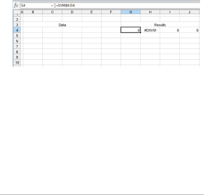
Data Management - 91 -

Note that Results can be a single cell, a single row, a single column, or a complete range.

If Results is a single cell, the width is determined by finding the first empty row to the right of the

Results cell. Then, the height is determined by finding the first row where all columns are empty.

If Results is a single row spanning multiple columns, the height of the range is determined by finding

the first row where all cells are empty.

If Results is a single column spanning multiple rows, the width of the range is determined by finding

the first column where all cells are empty.

If Results is a range with multiple rows and columns, no further expansion on the width or height is

done. The range is used as is.

In the template where the work is done, any data management function (with the exception of Result

from Template) can be configured as a connection. Every management connection configured must

have Active By set to a specific worksheet (do not use Any Sheet). Once all the management

connections are configured, click Export to export these to the Data Management worksheet within

the template. This sheet must be saved in the template as the Result from Template function executes

the management functions on this sheet. If, at a later date, management connections are added,

removed, or modified, click Export again to rebuild the worksheet.

Example

As a simple example, use a template to produce the total, average, minimum and maximum from a

range of data copied from a report and returning those summary calculation results.

In the template SummaryCalc, cell B4 is named Parameter1 and cells G4:J4 are named Results. To

expand the formulas in G4:J4, a Formula Range management function is configured as a connection.

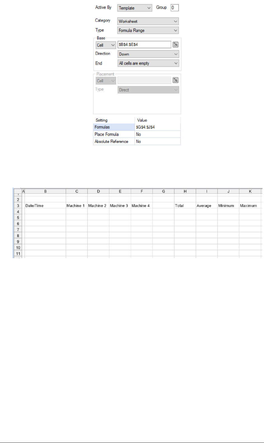
Data Management - 92 -

Once added and saved, the management connection is exported to the Data Management worksheet

and the SummaryCalc template is complete.

In the report template, a data connection is configured to retrieve the raw data from the historian and

an area has been dedicated to the results from the SummaryCalc template.

To get the summary data, the Result from Template management function is configured.

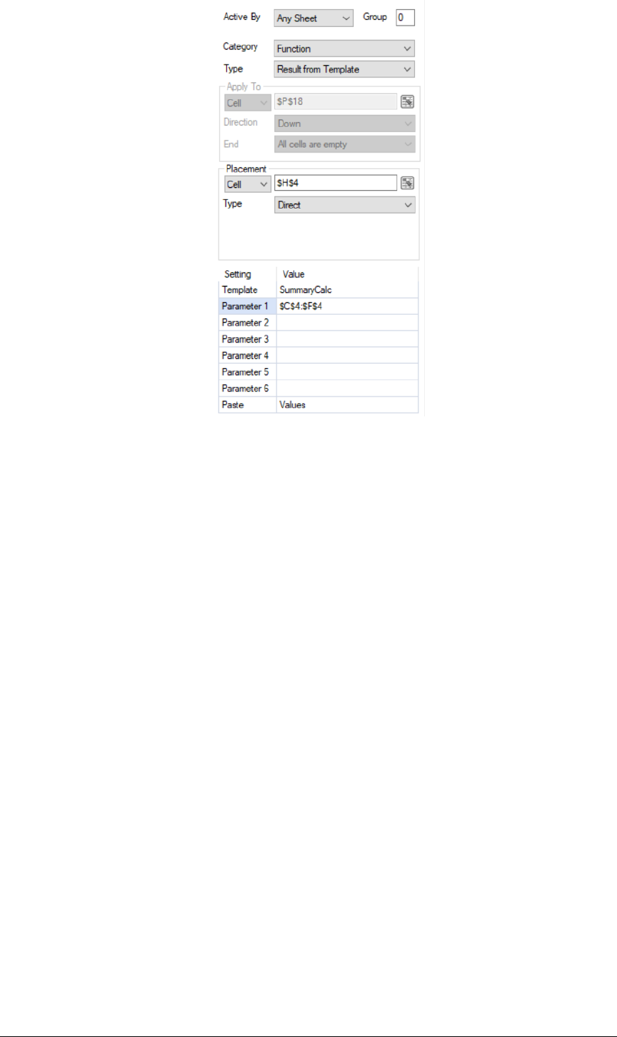
Data Management - 93 -

Note that Parameter 1 is set to $C$4:$F$4. When run, this range is expanded downwards until all the

cells between C and F are empty.

Settings

Template

The name of the template which contains the rules that determine the Results. This can be fixed

text or a cell reference.

If the file extension of the template is not specified, it is assumed to be the default set in the

project.

Parameter 1 – Parameter 6

Up to 6 parameters can be passed to the template. The values in these parameters are written into

the named cells Parameter1 – Parameter6 in the workbook specified.

These can be hard coded or cell references. If set to a cell reference, the cell reference is expanded

based on the data in the report.

If the parameter is a single cell the width is determined by finding the first empty row to the right

of the cell. Then, the height is determined by finding the first row where all columns are empty.

If the parameter is a single row spanning multiple columns, the height of the range is determined

by finding the first row where all cells are empty.

If the parameter is a single column spanning multiple rows, the width of the range is determined

by finding the first column where all cells are empty.

If the parameter is a range with multiple rows and columns, no further expansion on the width or

height is done. The range is used as is.

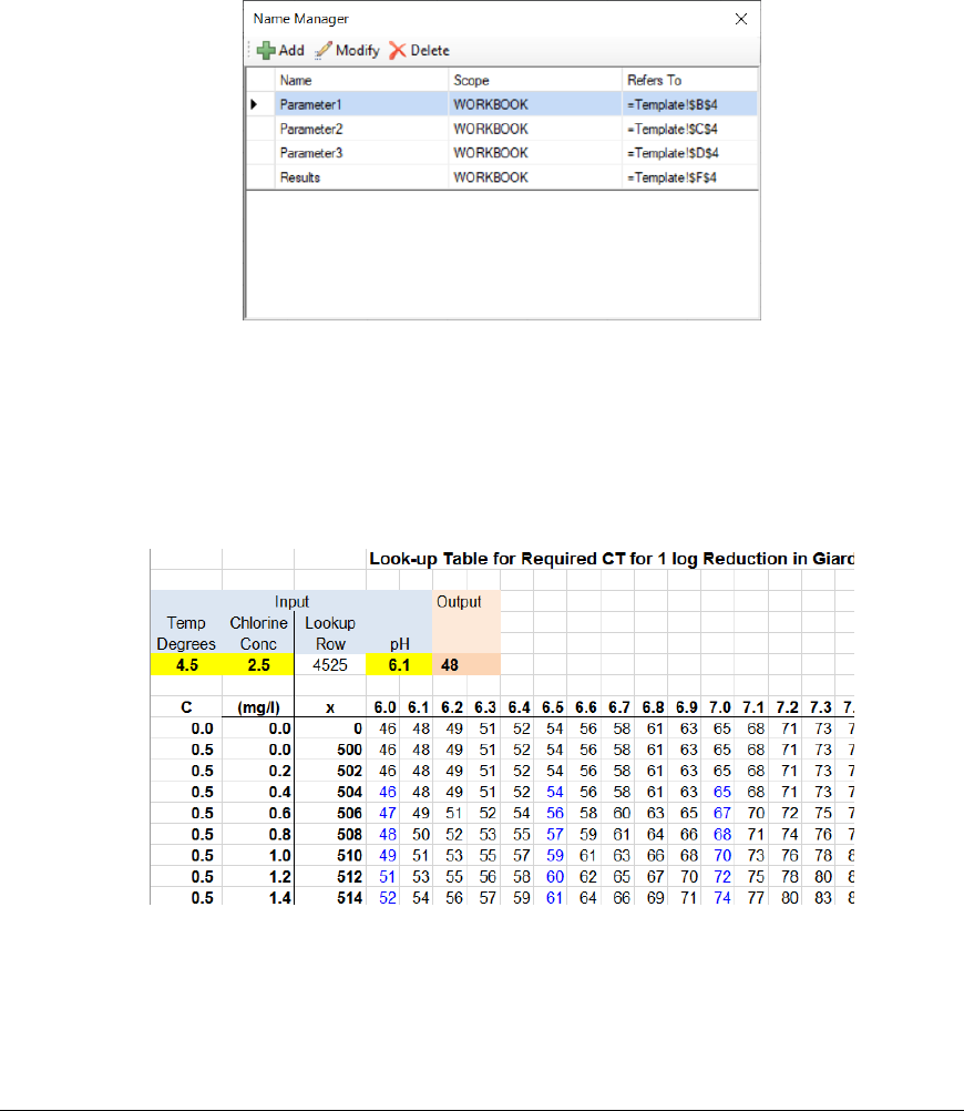
Data Management - 94 -

Paste

This setting determines what from the Results is copied back to the report. To use the formatting

from the template, select Values and Formats, otherwise select Values to use the formatting set in

the report template.

Result from Workbook

A powerful feature of workbooks is that they provide hundreds of formula/functions.

With complex formula rules, it may be preferable to express them in a workbook separate from the

report so that they can be used in every report without replication. The Result from Workbook

function is provided to copy parameters from the report to a separate workbook where complex

formulas operate on the data and return those results to the report.

In the separate workbook, named ranges are used to identify where up to 6 parameters are copied from

the report as well as where the results are located that are copied back to the report. Parameters are

designated with the names Parameter1 to Parameter6 and the results are designated with the name

Results.

Note that each parameter as well as Results can refer to either a single cell or a range and that the

Scope of each name must be set to WORKBOOK.

For more information on named ranges and cells see the Named Cells/Ranges section of the

Template Studio document under the DESIGN category in the Document Library.

For example, in water treatment, a lookup table is used to calculate giardia levels from chlorine,

temperature and pH. These tables are readily available from the EPA web site.

To make this suitable as a lookup to a report, each of the inputs and the output need to be identified.

The inputs (yellow) are given the names Parameter1, Parameter2 and Parameter3. The output cell is

given the name Results.

The formula for the output is similar to the following which uses the temperature, chlorine, and pH to

determine the result from the EPA lookup table:

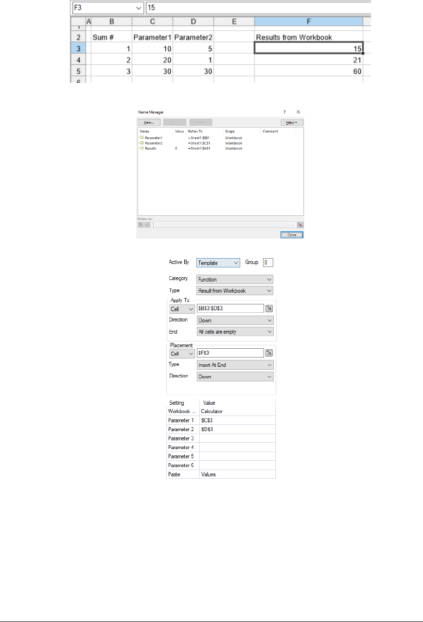
Data Management - 95 -

=VLOOKUP(C6, C8:AH425, MATCH(D6, C8:AH8,1))

Note that this workbook is provided in the XLReporter\_library\_Import directory as giardia-

lookup.xlsx

Example

As a simple example, use an external workbook to sum Parameter1 and Parameter2.

This configuration uses a Calculators workbook that has a Results, Parameter1, and Parameter2

Named Cells with the following declarations:

The Results cell contains a =Parameter1+Parameter2 formula.

Use the settings:

Apply To $B$3:$D$3, Down, All cells are empty

Placement $F$3, Insert At End, Down

Setting

Workbook Name Calculator

Parameter 1 $C$3

Parameter 2 $D$3

Parameter 3

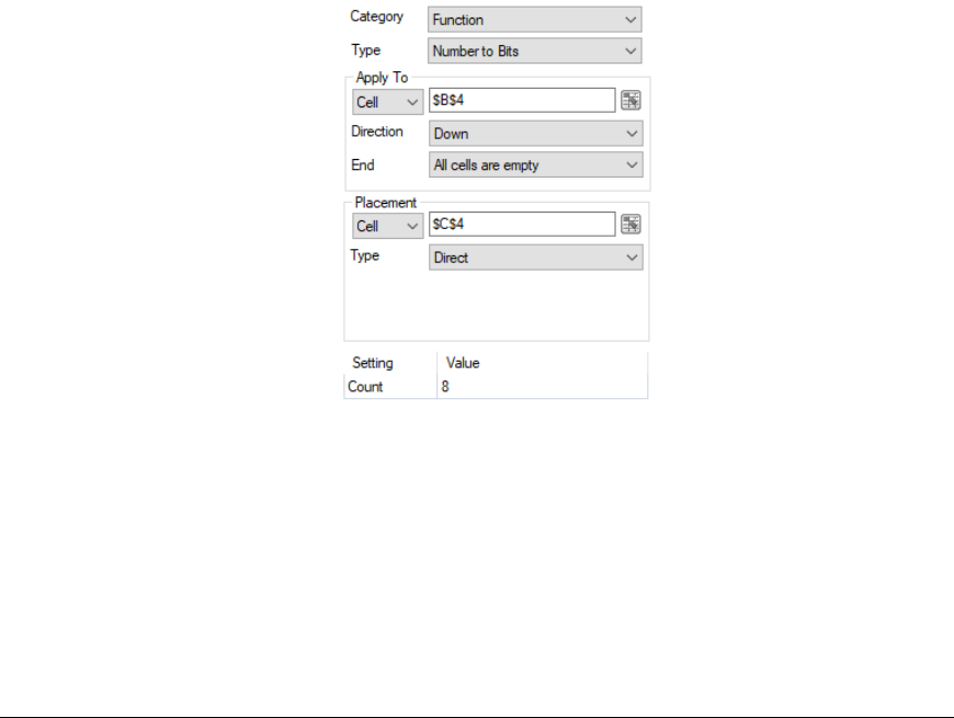
Data Management - 96 -

Parameter 4

Parameter 5

Parameter 6

Paste Values

Settings

Workbook Name

The name of the workbook which contains the rules that determine the Results. This can be fixed

text or a cell reference.

If the full path of the workbook is not specified, it is assumed that the workbook is in the Input

folder of the project. If the file extension of the workbook is not specified, it is assumed to be the

default set in the project.

Parameter 1 – Parameter 6

Up to 6 parameters can be passed to the workbook. The values in these parameters are written

into the named cells Parameter1 – Parameter6 in the workbook specified.

These can be hard coded or cell references. If set to a cell reference and the Apply To range spans

multiple rows, the row for the cell reference is adjusted as each row in the Apply To range is

processed.

Paste

This setting determines what from the Results is copied back to the report. To use the formatting

from the workbook, select Values and Formats, otherwise select Values to use the formatting set

in the template.

Number to Bits

Registers read from a PLC that represent a bitmask need to be expanded to their individual bits so as to

give meaning to the register value e.g., an alarm register representing which alarms are active.

The Apply To is the top row of the column containing the numbers to expand. The bit setting is

written to the Placement. The Count is the count of how many bits in the number will be used, e.g., a

value of 62 with a Count of 5 produces 11110.

Settings

Count

A count of how many bits in the number will be used. This value cannot exceed 63 so if the value

specified is greater than 63 it will be truncated.

Data Management - 97 -

Example

A motor has 8 possible alarms which are represented in the PLC as the bits of an integer register. A

change in the integer value causes the timestamp and value to be written in a new row starting in cells

$B$4 and $C$4.

The alarm bits can be expanded in rows starting in cell $E$4 with the following configured:

Placement

Apply To $C$4, Down, All Cells Empty

Placement $E$4, Direct

Setting

Count 8

Select Worksheet

The Select Worksheet function selects a worksheet in the report making it the visible worksheet when

the workbook is opened.

Settings

Worksheet

The name of the worksheet to select. This can be a fixed name or a cell reference where the cell

contains the name of the worksheet to select.

Range

The range to select on the Worksheet specified. This can be left blank if it is not needed.

Example

A monthly report workbook contains report worksheets for every day of the month as well as a

Summary worksheet containing daily summaries. The daily report worksheets are updated every day.

When a user views the monthly report workbook, the Summary worksheet should be selected.

In practice, the last updated sheet will be the one visible to the user when the workbook is opened

which is not what is required. Use this function with:

Settings

Worksheet Summary

Timestamp Convert

Timestamps from a data source sometimes needs to be converted to the requirement of the report. For

example, it is common to find timestamps in Coordinated Universal Time (UTC), which is the primary

time standard by which the world regulates clocks, needing to be converted into a local time.

This function converts cell values in the Apply To range based on the Format specified. The

converted timestamps are written based on the Placement settings. To overwrite the timestamps with

the converted, set the Placement cell to the top left corner of the Apply To range.

Settings

Format

The format to convert the timestamp to. The following are available:

Locale Time

Use this Format if the timestamps to convert are in UTC time and need to be converted to a

time in a specific Locale.

UTC Time

Use this Format if the timestamps to convert are in a time in a specific Locale and need to be

converted to UTC time.

Data Management - 98 -

Custom

Use this format to add or subtract from the timestamps. The Value and Unit settings are used

for this setting.

Locale

The time zone to convert the timestamp to (if Format is Locale Time) or to convert the timestamp

from (if Format is UTC Time).

If left blank this is assumed to be the time zone of the Windows OS.

A list of all supported Locale setting can be found in the text file timezones.txt. This is located in

the installation directory of the product (C:\XLReporter by default).

This setting can be a fixed time zone name or a cell reference. When set as a cell reference the

cell specified is the top row of a list of time zones that correspond to every row of data in the

Apply To range.

Value, Unit

The value to adjust the timestamp (positive or negative) in the unit specified.

Example

A report contains totals of the previous day, but the timestamps are from the current day. If the

timestamp is written to cell $B$4, it can be converted to the previous day as follows:

Placement

Apply To $B$4, None, All Cells Empty

Placement $B$4, Direct

Setting

Format Custom

Locale

Value 1

Unit Day

Trim Text

Some data sources can return textual data in a format that is not conducive to a report. For example,

text strings may be returned with a fixed length or padded with spaces, which in the report will not

display correctly.

This function trims the text from every cell in the Apply To range, writing the trimmed text to the

corresponding cell based on the Placement. To overwrite the original text with the trimmed text, set

the Placement cell to the top left corner of the Apply To range.

Settings

Text to Trim

Set to the text string to trim. A dropdown list provides some common characters to trim. The text

string to trim can also be entered directly in this setting.

Trim From

This determines from where the text is trimmed: from the Left, from the Right, or Both from the

left and right.

Data Management - 99 -

Example

A database table contains a column that is fixed to 32 characters which means that if any text is less

than 32 characters it has empty spaces to fill the remaining characters. This column of data starts in

cell $C$4. To trim the trailing spaces from these values:

Apply To $C$4, Down, All Cells Empty

Placement $C$4, Direct

Setting

Text to Trim Space

Trim From Right

Zero Pad

When displaying information like numeric product codes or batch IDs, it may be required to zero pad

these values so that each is a consistent length. If the values are delivered as numbers, this function

can zero pad them to a consistent length.

This function zero pads the value from every cell in the Apply To range, writing the zero-padded value

to the corresponding cell based on the Placement. To overwrite the original value with the zero-

padded value, set the Placement cell to the top left corner of the Apply To range.

Settings

Padding

This determines the maximum number of characters each value in the Apply To range is padded.

Example

The part number fabricated by a machine must always be 12 characters in length with 0’s padding any

part number less than 12 characters to be consistent. The report shows all the part numbers generated

over the day with the part number itself starting in cell $C$4. To zero pad these values in place:

Apply To $C$4, Down, All Cells Empty

Placement $C$4, Direct

Setting

Padding 12

Data Management - 100 -

Custom Category

Overview

XLReporter provides an interface for users to provide their own business logic in .NET classes.

A management function in a custom category behaves similar to other management functions except

that the input cell range together with the user specified parameters are passed to a .NET class for

processing. The result from the .NET class is positioned on the configured output cell.

This is an advanced feature and is described in more detail in the Generate Reports

Programmatically document found in the Document Library under the REPORT section.

Data Management - 101 -

Information in this document is subject to change without notice. SyTech assumes no responsibility for

any errors or omissions that may be in this document. No part of this document may be reproduced or

transmitted in any form or by any means, electronic or mechanical, for any purpose, without the prior

written permission of SyTech.

XLReporter

is a registered trademark of SyTech (dba of TheReportCompany, LLC).

Microsoft

and Microsoft Excel

are registered trademarks of Microsoft, Inc.

All registered names are the property of their respective owners.